Building Attributes for our Smoke Dataset

The Setup

You’ve now used the PurpleAir data a few times. A fairly obvious question seems to be how does an area’s particulate matter (PM2.5) burden coincide with it’s wildfire hazard. Similarly, how does the PM2.5 burden coincide with life expectancy. We’ll use our raster of wildfire hazard probability, our vector dataset of Climate and Environmental Justice, and the sensor data themselves to begin building a dataset that would allow us to explore this question.

Getting Started

First, we’ll have to get our credentials and login to a new RStudio session. You can create your own repository if you’d like to track these things. You’ll have to copy your googledrive download function from a previous repo.

I’ve added a few additional datasets to our Google Drive folder, so we’ll need to load packages, download our data, and get a few things setup before we start building.

First, let’s get our packages and our Google Drive download script loaded.

Code

library(googledrive)
library(terra)

terra 1.8.70

Code

library(sf)

Linking to GEOS 3.13.0, GDAL 3.8.5, PROJ 9.5.1; sf_use_s2() is TRUE

Code

library(tidyterra)

Attaching package: 'tidyterra'

The following object is masked from 'package:stats':

    filter

Code

library(tidyverse)

── Attaching core tidyverse packages ──────────────────────── tidyverse 2.0.0 ──
✔ dplyr     1.1.4     ✔ readr     2.1.5
✔ forcats   1.0.1     ✔ stringr   1.5.2
✔ ggplot2   4.0.0     ✔ tibble    3.3.0
✔ lubridate 1.9.4     ✔ tidyr     1.3.1
✔ purrr     1.1.0     

── Conflicts ────────────────────────────────────────── tidyverse_conflicts() ──
✖ tidyr::extract() masks terra::extract()
✖ dplyr::filter()  masks tidyterra::filter(), stats::filter()
✖ dplyr::lag()     masks stats::lag()
ℹ Use the conflicted package (<http://conflicted.r-lib.org/>) to force all conflicts to become errors

Code

source("scripts/utilities/download_utils.R")

Checking Data, Allignment, and Choosing Variables

Let’s download everything in our folder

Code

file_list <- drive_ls(drive_get(as_id("https://drive.google.com/drive/u/1/folders/1PwfUX2hnJlbnqBe3qvl33tFBImtNFTuR")))[-1,]

! Using an auto-discovered, cached token.

  To suppress this message, modify your code or options to clearly consent to
  the use of a cached token.

  See gargle's "Non-interactive auth" vignette for more details:

  <https://gargle.r-lib.org/articles/non-interactive-auth.html>

ℹ The googledrive package is using a cached token for
  'mattwilliamson@boisestate.edu'.

Code

file_list %>% 
  dplyr::select(id, name) %>%
  purrr::pmap(function(id, name) {
    gdrive_folder_download(list(id = id, name = name),
                           dstfldr = "inclass09")
  })

File downloaded:

• 'blockgroupPop.shx' <id: 10RKLXNzoNfYQralSDDbsAkxgwSGgc46w>

Saved locally as:

• 'data/original/inclass09/blockgroupPop.shx'

File downloaded:

• 'blockgroupPop.shp' <id: 19HSGozYvuqmXQ-CtPVkwFcFmDK-V6aIr>

Saved locally as:

• 'data/original/inclass09/blockgroupPop.shp'

File downloaded:

• 'blockgroupPop.dbf' <id: 14alTpZHGZ067Ez1270Q7ffiVKO4zbY3p>

Saved locally as:

• 'data/original/inclass09/blockgroupPop.dbf'

File downloaded:

• 'blockgroupPop.prj' <id: 1QbV7Dn53zM_KvuUKc7rBug9R5lRg3rFy>

Saved locally as:

• 'data/original/inclass09/blockgroupPop.prj'

File downloaded:

• 'paReadings.csv' <id: 184wxWw1DQrllUAFUnXtR0TSMYVqWUJ_G>

Saved locally as:

• 'data/original/inclass09/paReadings.csv'

File downloaded:

• 'pa_pt_locations.shx' <id: 14rFc7Hxgxl6QfuhfYtRDvNE6TOYUnho4>

Saved locally as:

• 'data/original/inclass09/pa.shx'

File downloaded:

• 'pa_pt_locations.shp' <id: 15zHbHjWhcuxT0sgOuElDAh1QgOYEbjZN>

Saved locally as:

• 'data/original/inclass09/pa.shp'

File downloaded:

• 'pa_pt_locations.dbf' <id: 13yZY6gkyd7GT7MVL5vOwI8xMcPCCZrTs>

Saved locally as:

• 'data/original/inclass09/pa.dbf'

File downloaded:

• 'pa_pt_locations.prj' <id: 1yC1NjbbrbWAMiiJjcTobzfg252ah-pek>

Saved locally as:

• 'data/original/inclass09/pa.prj'

File downloaded:

• 'pa_censors_loc.csv' <id: 13ZPu8E96ERWdUNlwQ5MB_vXrPCqvzxj_>

Saved locally as:

• 'data/original/inclass09/pa.csv'

File downloaded:

• 'wildfire_hazard_agg.tif' <id: 135PvMlKu17i7tZcrF7XiWxzrzaX-aCLn>

Saved locally as:

• 'data/original/inclass09/wildfire.tif'

File downloaded:

• 'cejst_nw.shx' <id: 1IXDayQ35MwCfq1UtuDHCtf5iNYq5VUqu>

Saved locally as:

• 'data/original/inclass09/cejst.shx'

File downloaded:

• 'cejst_nw.dbf' <id: 1PgCOsZsVEOhxQs2Dpz21MNz0kMb32amB>

Saved locally as:

• 'data/original/inclass09/cejst.dbf'

File downloaded:

• 'cejst_nw.shp' <id: 1ZeL_683mTTWdCDjQ4dY6oJsxyVZtQT6O>

Saved locally as:

• 'data/original/inclass09/cejst.shp'

File downloaded:

• 'cejst_nw.prj' <id: 1r7OHK1DHhoEMBToiM2FmuK5xmEzWSdrc>

Saved locally as:

• 'data/original/inclass09/cejst.prj'

[[1]]
[1] "data/original/inclass09/blockgroupPop.shx"

[[2]]
[1] "data/original/inclass09/blockgroupPop.shp"

[[3]]
[1] "data/original/inclass09/blockgroupPop.dbf"

[[4]]
[1] "data/original/inclass09/blockgroupPop.prj"

[[5]]
[1] "data/original/inclass09/paReadings.csv"

[[6]]
[1] "data/original/inclass09/pa.shx"

[[7]]
[1] "data/original/inclass09/pa.shp"

[[8]]
[1] "data/original/inclass09/pa.dbf"

[[9]]
[1] "data/original/inclass09/pa.prj"

[[10]]
[1] "data/original/inclass09/pa.csv"

[[11]]
[1] "data/original/inclass09/wildfire.tif"

[[12]]
[1] "data/original/inclass09/cejst.shx"

[[13]]
[1] "data/original/inclass09/cejst.dbf"

[[14]]
[1] "data/original/inclass09/cejst.shp"

[[15]]
[1] "data/original/inclass09/cejst.prj"

Let’s load our spatial data and see what we’ve got! We’ll start by checking the CRS for each of the datasets.

Code

cejst_shp <- read_sf("data/original/inclass09/cejst.shp")

fire_prob <- rast("data/original/inclass09/wildfire.tif")

pa_locations_wgs <- read_sf("data/original/inclass09/pa.shp")

st_crs(cejst_shp)

Coordinate Reference System:
  User input: WGS 84 
  wkt:
GEOGCRS["WGS 84",
    DATUM["World Geodetic System 1984",
        ELLIPSOID["WGS 84",6378137,298.257223563,
            LENGTHUNIT["metre",1]]],
    PRIMEM["Greenwich",0,
        ANGLEUNIT["degree",0.0174532925199433]],
    CS[ellipsoidal,2],
        AXIS["latitude",north,
            ORDER[1],
            ANGLEUNIT["degree",0.0174532925199433]],
        AXIS["longitude",east,
            ORDER[2],
            ANGLEUNIT["degree",0.0174532925199433]],
    ID["EPSG",4326]]

Code

st_crs(pa_locations_wgs)

Coordinate Reference System:
  User input: NAD83 
  wkt:
GEOGCRS["NAD83",
    DATUM["North American Datum 1983",
        ELLIPSOID["GRS 1980",6378137,298.257222101,
            LENGTHUNIT["metre",1]]],
    PRIMEM["Greenwich",0,
        ANGLEUNIT["degree",0.0174532925199433]],
    CS[ellipsoidal,2],
        AXIS["latitude",north,
            ORDER[1],
            ANGLEUNIT["degree",0.0174532925199433]],
        AXIS["longitude",east,
            ORDER[2],
            ANGLEUNIT["degree",0.0174532925199433]],
    ID["EPSG",4269]]

Code

crs(fire_prob)

[1] "PROJCRS[\"unnamed\",\n    BASEGEOGCRS[\"NAD83\",\n        DATUM[\"North American Datum 1983\",\n            ELLIPSOID[\"GRS 1980\",6378137,298.257222101004,\n                LENGTHUNIT[\"metre\",1]]],\n        PRIMEM[\"Greenwich\",0,\n            ANGLEUNIT[\"degree\",0.0174532925199433]],\n        ID[\"EPSG\",4269]],\n    CONVERSION[\"Albers Equal Area\",\n        METHOD[\"Albers Equal Area\",\n            ID[\"EPSG\",9822]],\n        PARAMETER[\"Latitude of false origin\",23,\n            ANGLEUNIT[\"degree\",0.0174532925199433],\n            ID[\"EPSG\",8821]],\n        PARAMETER[\"Longitude of false origin\",-96,\n            ANGLEUNIT[\"degree\",0.0174532925199433],\n            ID[\"EPSG\",8822]],\n        PARAMETER[\"Latitude of 1st standard parallel\",29.5,\n            ANGLEUNIT[\"degree\",0.0174532925199433],\n            ID[\"EPSG\",8823]],\n        PARAMETER[\"Latitude of 2nd standard parallel\",45.5,\n            ANGLEUNIT[\"degree\",0.0174532925199433],\n            ID[\"EPSG\",8824]],\n        PARAMETER[\"Easting at false origin\",0,\n            LENGTHUNIT[\"metre\",1],\n            ID[\"EPSG\",8826]],\n        PARAMETER[\"Northing at false origin\",0,\n            LENGTHUNIT[\"metre\",1],\n            ID[\"EPSG\",8827]]],\n    CS[Cartesian,2],\n        AXIS[\"easting\",east,\n            ORDER[1],\n            LENGTHUNIT[\"metre\",1,\n                ID[\"EPSG\",9001]]],\n        AXIS[\"northing\",north,\n            ORDER[2],\n            LENGTHUNIT[\"metre\",1,\n                ID[\"EPSG\",9001]]]]"

You’ll notice that we’ve got some slightly different projections. Let’s fix that before we get too far down the road. We’ll reproject the shapefiles as that’s the safest way to get everything lined up.

Code

cejst_reproj <- cejst_shp %>% 
  st_transform(., crs = crs(fire_prob))

pa_reproj <- pa_locations_wgs %>% 
  st_transform(., crs = crs(fire_prob))

Ok, now that we’ve gotten all of our spatial data lined up. Let’s load the last dataset, which is the tabular data depicting all of the monthly sensor readings. Let’s take a glimpse at all of the data.

Code

pa_data <- read_csv("data/original/inclass09/paReadings.csv")

Rows: 5945 Columns: 6
── Column specification ────────────────────────────────────────────────────────
Delimiter: ","
dbl  (5): id, humidity, temperature, pm2.5_atm, pm2.5_cf_1
dttm (1): time_stamp

ℹ Use `spec()` to retrieve the full column specification for this data.
ℹ Specify the column types or set `show_col_types = FALSE` to quiet this message.

Code

glimpse(cejst_reproj)

Rows: 2,590
Columns: 124
$ GEOID10    <chr> "16019970700", "16025970100", "16027021700", "16027020700",…
$ SF         <chr> "Idaho", "Idaho", "Idaho", "Idaho", "Idaho", "Idaho", "Idah…
$ CF         <chr> "Bonneville County", "Camas County", "Canyon County", "Cany…
$ DF_PFS     <dbl> 0.44, 0.67, 0.74, 0.48, 0.75, 0.80, 0.76, 0.72, 0.76, 0.52,…
$ AF_PFS     <dbl> 0.73, 0.65, 0.86, 0.63, 0.79, 0.88, 0.86, 0.79, 0.80, 0.65,…
$ HDF_PFS    <dbl> 0.57, 0.79, 0.69, 0.47, 0.72, 0.55, 0.53, 0.71, 0.74, 0.45,…
$ DSF_PFS    <dbl> 0.53, 0.00, 0.58, 0.46, 0.12, 0.79, 0.68, 0.27, 0.06, 0.11,…
$ EBF_PFS    <dbl> 0.63, 0.95, 0.54, 0.30, 0.63, 0.81, 0.81, 0.44, 0.73, 0.52,…
$ EALR_PFS   <dbl> 0.55, 0.83, 0.63, 0.63, 0.65, NA, 0.41, 0.64, 0.65, 0.64, 0…
$ EBLR_PFS   <dbl> 0.19, 0.93, 0.05, 0.55, 0.09, 0.09, 0.08, 0.09, 0.47, 0.17,…
$ EPLR_PFS   <dbl> 0.80, 0.99, 0.09, 0.10, 0.11, 0.31, 0.08, 0.09, 0.10, 0.09,…
$ HBF_PFS    <dbl> 0.69, 0.60, 0.53, 0.07, 0.46, 0.86, 0.93, 0.22, 0.53, 0.28,…
$ LLEF_PFS   <dbl> 0.73, 0.48, 0.67, 0.29, 0.51, 0.87, 0.62, 0.38, 0.32, 0.26,…
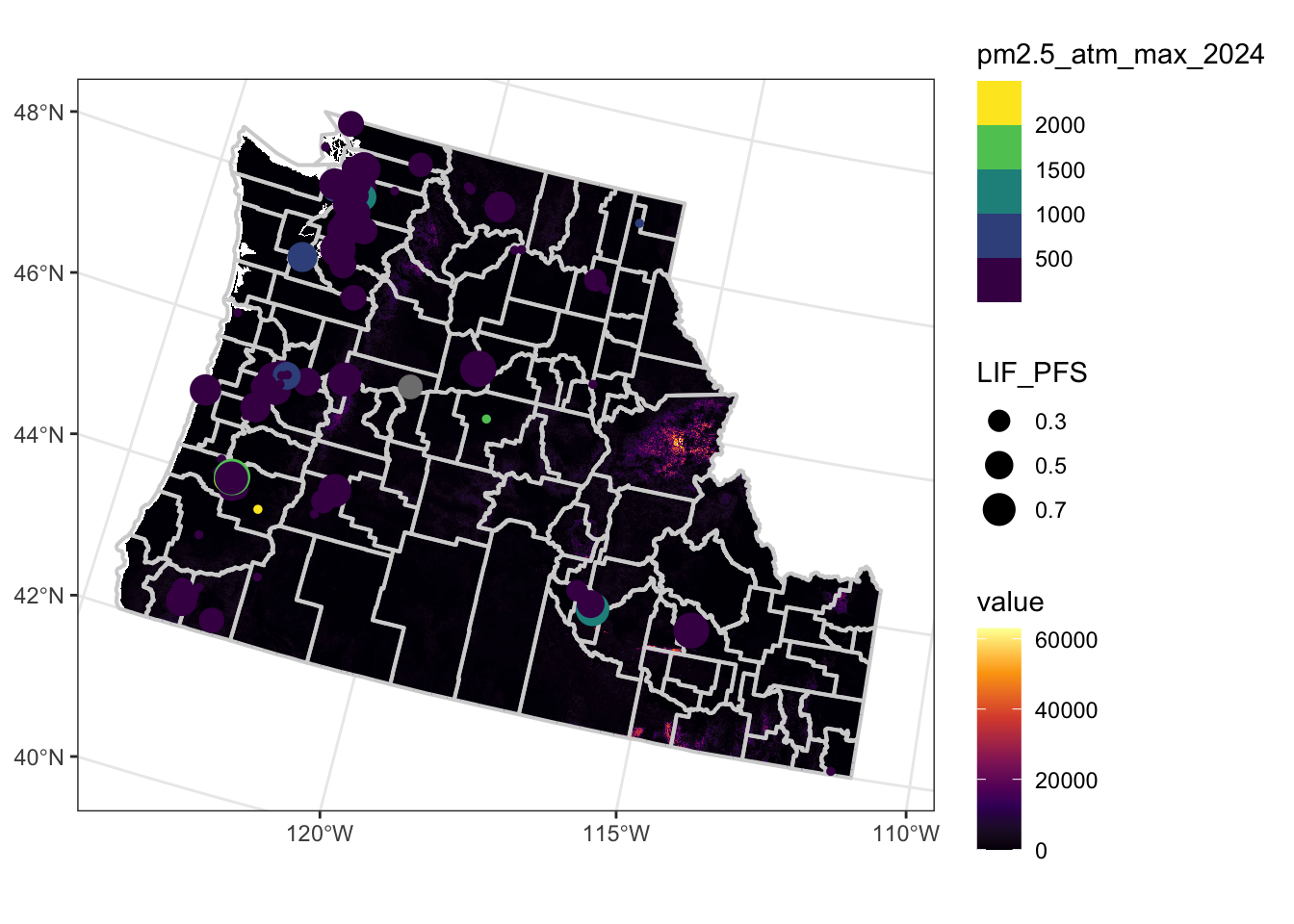
$ LIF_PFS    <dbl> 0.54, 0.54, 0.53, 0.12, 0.48, 0.61, 0.88, 0.46, 0.41, 0.32,…
$ LMI_PFS    <dbl> 0.81, 0.75, 0.61, 0.25, 0.55, 0.92, 0.95, 0.44, 0.42, 0.35,…
$ PM25F_PFS  <dbl> 0.11, 0.00, 0.68, 0.63, 0.42, 0.66, 0.69, 0.57, 0.26, 0.40,…
$ HSEF       <dbl> 0.14, 0.06, 0.20, 0.08, 0.21, 0.24, 0.31, 0.18, 0.18, 0.09,…
$ P100_PFS   <dbl> 0.83, 0.63, 0.47, 0.24, 0.60, 0.72, 0.93, 0.27, 0.39, 0.33,…
$ P200_I_PFS <dbl> 0.86, 0.71, 0.81, 0.39, 0.75, 0.98, 0.91, 0.49, 0.67, 0.54,…
$ AJDLI_ET   <int> 1, 1, 1, 0, 1, 1, 1, 0, 1, 1, 0, 1, 1, 1, 0, 0, 1, 0, 0, 0,…
$ LPF_PFS    <dbl> 0.75, 0.52, 0.26, 0.30, 0.65, 0.62, 0.63, 0.40, 0.51, 0.36,…
$ KP_PFS     <dbl> 0.86, 0.21, 0.84, 0.21, 0.61, 0.57, 0.21, 0.43, 0.90, 0.21,…
$ NPL_PFS    <dbl> 0.09, 0.05, 0.06, 0.08, 0.03, 0.08, 0.05, 0.05, 0.08, 0.10,…
$ RMP_PFS    <dbl> 0.49, 0.01, 0.56, 0.84, 0.26, 0.96, 0.58, 0.36, 0.10, 0.20,…
$ TSDF_PFS   <dbl> 0.22, 0.01, 0.14, 0.42, 0.07, 0.55, 0.13, 0.11, 0.10, 0.19,…
$ TPF        <dbl> 5589, 1048, 11701, 3901, 5059, 4681, 3006, 7423, 6653, 4693…
$ TF_PFS     <dbl> 0.55, 0.06, 0.54, 0.53, 0.28, 0.71, 0.83, 0.24, 0.05, 0.09,…
$ UF_PFS     <dbl> 0.61, 0.16, 0.64, 0.33, 0.66, 0.86, 0.80, 0.45, 0.47, 0.61,…
$ WF_PFS     <dbl> 0.03, 0.11, 0.98, 0.24, 0.79, 0.98, 0.98, 0.85, 0.42, 0.04,…
$ UST_PFS    <dbl> 0.59, 0.02, 0.44, 0.31, 0.17, 0.73, 0.83, 0.13, 0.06, 0.18,…
$ N_WTR      <int> 0, 0, 1, 0, 0, 1, 1, 0, 0, 0, 0, 0, 0, 0, 0, 0, 0, 0, 0, 0,…
$ N_WKFC     <int> 0, 0, 0, 0, 0, 1, 1, 0, 0, 0, 0, 0, 0, 0, 0, 0, 0, 0, 0, 0,…
$ N_CLT      <int> 0, 1, 0, 0, 0, 1, 1, 0, 0, 0, 0, 1, 0, 0, 0, 0, 0, 0, 0, 0,…
$ N_ENY      <int> 0, 1, 0, 0, 0, 0, 0, 0, 0, 0, 0, 1, 0, 0, 0, 0, 0, 0, 0, 0,…
$ N_TRN      <int> 0, 0, 0, 0, 0, 0, 0, 0, 1, 0, 0, 0, 0, 0, 0, 0, 1, 0, 0, 0,…
$ N_HSG      <int> 0, 0, 0, 0, 0, 0, 1, 0, 1, 0, 0, 1, 0, 0, 0, 0, 0, 0, 0, 0,…
$ N_PLN      <int> 0, 0, 0, 0, 0, 1, 0, 0, 0, 0, 0, 0, 0, 0, 0, 0, 0, 0, 0, 0,…
$ N_HLTH     <int> 0, 0, 0, 0, 0, 0, 0, 0, 0, 0, 0, 0, 0, 0, 0, 0, 0, 0, 0, 0,…
$ SN_C       <int> 0, 1, 1, 0, 0, 1, 1, 0, 1, 0, 0, 1, 0, 0, 0, 0, 1, 0, 0, 0,…
$ SN_T       <chr> NA, NA, NA, NA, NA, NA, NA, NA, NA, NA, NA, NA, NA, NA, NA,…
$ DLI        <int> 0, 0, 0, 0, 0, 0, 0, 0, 0, 0, 0, 0, 0, 0, 0, 0, 0, 0, 0, 0,…
$ ALI        <int> 0, 0, 0, 0, 0, 0, 0, 0, 0, 0, 0, 0, 0, 0, 0, 0, 0, 0, 0, 0,…
$ PLHSE      <int> 0, 0, 0, 0, 0, 0, 1, 0, 0, 0, 0, 0, 0, 0, 0, 0, 0, 0, 0, 0,…
$ LMILHSE    <int> 0, 0, 0, 0, 0, 1, 1, 0, 0, 0, 0, 0, 0, 0, 0, 0, 0, 0, 0, 0,…
$ ULHSE      <int> 0, 0, 0, 0, 0, 0, 0, 0, 0, 0, 0, 0, 0, 0, 0, 0, 0, 0, 0, 0,…
$ EPL_ET     <int> 0, 1, 0, 0, 0, 0, 0, 0, 0, 0, 0, 0, 0, 0, 0, 0, 0, 0, 0, 0,…
$ EAL_ET     <int> 0, 0, 0, 0, 0, 0, 0, 0, 0, 0, 0, 1, 0, 0, 0, 0, 0, 0, 0, 0,…
$ EBL_ET     <int> 0, 1, 0, 0, 0, 0, 0, 0, 0, 0, 0, 0, 0, 0, 0, 0, 0, 0, 0, 0,…
$ EB_ET      <int> 0, 1, 0, 0, 0, 0, 0, 0, 0, 0, 0, 1, 0, 0, 0, 0, 0, 0, 0, 0,…
$ PM25_ET    <int> 0, 0, 0, 0, 0, 0, 0, 0, 0, 0, 0, 0, 0, 0, 0, 0, 0, 0, 0, 0,…
$ DS_ET      <int> 0, 0, 0, 0, 0, 0, 0, 0, 0, 0, 0, 0, 0, 0, 0, 0, 0, 0, 0, 0,…
$ TP_ET      <int> 0, 0, 0, 0, 0, 0, 0, 0, 0, 0, 0, 0, 0, 0, 0, 0, 0, 0, 0, 0,…
$ LPP_ET     <int> 0, 0, 0, 0, 0, 0, 0, 0, 0, 0, 0, 0, 0, 0, 0, 0, 0, 0, 0, 0,…
$ HRS_ET     <chr> NA, NA, NA, NA, NA, NA, NA, NA, NA, NA, NA, NA, NA, NA, NA,…
$ KP_ET      <int> 0, 0, 0, 0, 0, 0, 0, 0, 1, 0, 0, 1, 0, 0, 0, 0, 0, 1, 0, 0,…
$ HB_ET      <int> 0, 0, 0, 0, 0, 0, 1, 0, 0, 0, 0, 0, 0, 0, 0, 0, 0, 0, 0, 0,…
$ RMP_ET     <int> 0, 0, 0, 0, 0, 1, 0, 0, 0, 0, 0, 0, 0, 0, 0, 0, 0, 0, 0, 0,…
$ NPL_ET     <int> 0, 0, 0, 0, 0, 0, 0, 0, 0, 0, 0, 0, 0, 0, 0, 0, 0, 0, 0, 0,…
$ TSDF_ET    <int> 0, 0, 0, 0, 0, 0, 0, 0, 0, 0, 0, 0, 0, 0, 0, 0, 0, 0, 0, 0,…
$ WD_ET      <int> 0, 0, 1, 0, 0, 1, 1, 0, 0, 0, 0, 0, 0, 0, 0, 0, 0, 0, 0, 0,…
$ UST_ET     <int> 0, 0, 0, 0, 0, 0, 0, 0, 0, 0, 0, 0, 0, 0, 0, 0, 0, 0, 0, 0,…
$ DB_ET      <int> 0, 0, 0, 0, 0, 0, 0, 0, 0, 0, 0, 0, 0, 0, 0, 0, 0, 0, 0, 0,…
$ A_ET       <int> 0, 0, 0, 0, 0, 0, 0, 0, 0, 0, 0, 0, 0, 0, 0, 0, 0, 0, 0, 0,…
$ HD_ET      <int> 0, 0, 0, 0, 0, 0, 0, 0, 0, 0, 0, 0, 0, 0, 0, 0, 0, 0, 0, 0,…
$ LLE_ET     <int> 0, 0, 0, 0, 0, 0, 0, 0, 0, 0, 0, 0, 0, 0, 0, 0, 0, 0, 0, 0,…
$ UN_ET      <int> 0, 0, 0, 0, 0, 0, 0, 0, 0, 0, 0, 0, 0, 0, 0, 0, 0, 0, 0, 0,…
$ LISO_ET    <int> 0, 0, 0, 0, 0, 0, 0, 0, 0, 0, 0, 0, 0, 0, 0, 0, 0, 0, 0, 0,…
$ POV_ET     <int> 0, 0, 0, 0, 0, 0, 1, 0, 0, 0, 0, 0, 0, 0, 0, 0, 0, 0, 0, 0,…
$ LMI_ET     <int> 0, 0, 0, 0, 0, 1, 1, 0, 0, 0, 0, 0, 0, 0, 0, 0, 0, 0, 0, 0,…
$ IA_LMI_ET  <int> 0, 0, 0, 0, 0, 0, 0, 0, 0, 0, 0, 0, 0, 0, 0, 0, 0, 0, 0, 0,…
$ IA_UN_ET   <int> 0, 0, 0, 0, 0, 0, 0, 0, 0, 0, 0, 0, 0, 0, 0, 0, 0, 0, 0, 0,…
$ IA_POV_ET  <int> 0, 0, 0, 0, 0, 0, 0, 0, 0, 0, 0, 0, 0, 0, 0, 0, 0, 0, 0, 0,…
$ TC         <dbl> 0, 3, 1, 0, 0, 4, 5, 0, 2, 0, 0, 3, 0, 0, 0, 0, 1, 0, 0, 0,…
$ CC         <dbl> 0, 2, 1, 0, 0, 4, 4, 0, 2, 0, 0, 3, 0, 0, 0, 0, 1, 0, 0, 0,…
$ IAULHSE    <int> 0, 0, 0, 0, 0, 0, 0, 0, 0, 0, 0, 0, 0, 0, 0, 0, 0, 0, 0, 0,…
$ IAPLHSE    <int> 0, 0, 0, 0, 0, 0, 0, 0, 0, 0, 0, 0, 0, 0, 0, 0, 0, 0, 0, 0,…
$ IALMILHSE  <int> 0, 0, 0, 0, 0, 0, 0, 0, 0, 0, 0, 0, 0, 0, 0, 0, 0, 0, 0, 0,…
$ IALMIL_76  <dbl> NA, NA, NA, NA, NA, NA, NA, NA, NA, NA, NA, NA, NA, NA, NA,…
$ IAPLHS_77  <dbl> NA, NA, NA, NA, NA, NA, NA, NA, NA, NA, NA, NA, NA, NA, NA,…
$ IAULHS_78  <dbl> NA, NA, NA, NA, NA, NA, NA, NA, NA, NA, NA, NA, NA, NA, NA,…
$ LHE        <int> 1, 0, 1, 0, 1, 1, 1, 1, 1, 0, 0, 1, 0, 0, 0, 0, 0, 0, 0, 0,…
$ IALHE      <int> 0, 0, 0, 0, 0, 0, 0, 0, 0, 0, 0, 0, 0, 0, 0, 0, 0, 0, 0, 0,…
$ IAHSEF     <dbl> NA, NA, NA, NA, NA, NA, NA, NA, NA, NA, NA, NA, NA, NA, NA,…
$ N_CLT_EOMI <int> 0, 1, 0, 0, 0, 1, 1, 0, 0, 0, 0, 1, 0, 0, 0, 0, 0, 0, 0, 0,…
$ N_ENY_EOMI <int> 0, 1, 0, 0, 0, 0, 0, 0, 0, 0, 0, 1, 0, 0, 0, 0, 0, 0, 0, 0,…
$ N_TRN_EOMI <int> 0, 0, 0, 0, 0, 0, 0, 1, 1, 0, 0, 0, 0, 0, 0, 0, 1, 0, 0, 0,…
$ N_HSG_EOMI <int> 0, 0, 0, 0, 0, 0, 1, 0, 1, 0, 0, 1, 0, 0, 0, 0, 0, 0, 0, 0,…
$ N_PLN_EOMI <int> 0, 0, 0, 0, 0, 1, 0, 0, 0, 0, 0, 0, 0, 0, 0, 0, 0, 0, 0, 0,…
$ N_WTR_EOMI <int> 0, 0, 1, 0, 0, 1, 1, 0, 0, 0, 0, 0, 0, 0, 0, 0, 0, 0, 0, 0,…
$ N_HLTH_88  <int> 0, 0, 0, 0, 0, 0, 0, 0, 0, 0, 0, 0, 0, 0, 0, 0, 0, 0, 0, 0,…
$ N_WKFC_89  <int> 0, 0, 0, 0, 0, 1, 1, 0, 0, 0, 0, 0, 0, 0, 0, 0, 0, 0, 0, 0,…
$ FPL200S    <int> 1, 1, 1, 0, 1, 1, 1, 0, 1, 0, 0, 1, 0, 0, 0, 0, 1, 0, 0, 0,…
$ N_WKFC_91  <int> 1, 0, 1, 0, 1, 1, 1, 1, 1, 0, 0, 1, 0, 0, 0, 0, 0, 0, 0, 0,…
$ TD_ET      <int> 0, 0, 0, 0, 0, 0, 0, 1, 1, 0, 0, 0, 0, 0, 0, 0, 1, 0, 0, 0,…
$ TD_PFS     <dbl> 0.67, 0.78, 0.60, 0.63, 0.85, 0.35, 0.29, 0.94, 0.91, 0.78,…
$ FLD_PFS    <dbl> 0.83, 0.88, 0.43, 0.24, 0.82, 0.93, 0.97, 0.44, 0.49, 0.71,…
$ WFR_PFS    <dbl> 0.70, 0.82, 0.33, 0.87, 0.80, 0.33, 0.83, 0.77, 0.81, 0.78,…
$ FLD_ET     <int> 0, 0, 0, 0, 0, 1, 1, 0, 0, 0, 0, 0, 0, 0, 0, 0, 0, 0, 0, 0,…
$ WFR_ET     <int> 0, 0, 0, 0, 0, 0, 0, 0, 0, 0, 0, 0, 0, 0, 0, 0, 0, 0, 0, 0,…
$ ADJ_ET     <int> 0, 0, 0, 0, 0, 1, 0, 0, 0, 0, 0, 0, 0, 0, 0, 0, 0, 0, 0, 0,…
$ IS_PFS     <dbl> 0.64, 0.16, 0.41, 0.53, 0.86, 0.46, 0.51, 0.70, 0.82, 0.86,…
$ IS_ET      <int> 0, 0, 0, 0, 0, 0, 0, 0, 0, 0, 1, 0, 1, 0, 1, 0, 0, 0, 0, 1,…
$ AML_ET     <int> 0, 0, 0, 0, 0, 0, 0, 0, 0, 0, 0, 0, 0, 0, 0, 0, 0, 0, 0, 0,…
$ FUDS_RAW   <chr> NA, NA, NA, NA, NA, NA, NA, NA, "0", NA, NA, NA, NA, NA, NA…
$ FUDS_ET    <int> 0, 0, 0, 0, 0, 0, 0, 0, 0, 0, 0, 0, 0, 0, 0, 0, 0, 0, 0, 0,…
$ IMP_FLG    <chr> "0", "0", "0", "0", "0", "0", "0", "0", "0", "0", "0", "0",…
$ DM_B       <dbl> 0.04, 0.00, 0.00, 0.00, 0.00, 0.00, 0.00, 0.00, 0.00, 0.01,…
$ DM_AI      <dbl> 0.01, 0.00, 0.01, 0.00, 0.00, 0.02, 0.01, 0.00, 0.00, 0.00,…
$ DM_A       <dbl> 0.00, 0.00, 0.00, 0.01, 0.00, 0.00, 0.00, 0.00, 0.00, 0.00,…
$ DM_HI      <dbl> 0.00, 0.00, 0.01, 0.00, 0.00, 0.00, 0.00, 0.00, 0.00, 0.00,…
$ DM_T       <dbl> 0.06, 0.00, 0.06, 0.04, 0.04, 0.06, 0.03, 0.01, 0.02, 0.00,…
$ DM_W       <dbl> 0.62, 0.98, 0.59, 0.88, 0.71, 0.54, 0.40, 0.81, 0.83, 0.85,…
$ DM_H       <dbl> 0.27, 0.01, 0.36, 0.07, 0.26, 0.42, 0.54, 0.16, 0.15, 0.11,…
$ DM_O       <dbl> 0.11, 0.00, 0.15, 0.02, 0.11, 0.12, 0.27, 0.03, 0.02, 0.02,…
$ AGE_10     <dbl> 0.18, 0.16, 0.15, 0.12, 0.12, 0.15, 0.17, 0.10, 0.10, 0.14,…
$ AGE_MIDDLE <dbl> 0.71, 0.65, 0.71, 0.71, 0.68, 0.77, 0.72, 0.71, 0.76, 0.66,…
$ AGE_OLD    <dbl> 0.10, 0.18, 0.13, 0.15, 0.18, 0.07, 0.09, 0.18, 0.12, 0.18,…
$ TA_COU_116 <dbl> NA, NA, NA, NA, NA, NA, NA, NA, NA, NA, NA, NA, NA, NA, NA,…
$ TA_COUNT_C <dbl> NA, NA, NA, NA, NA, NA, NA, NA, NA, NA, NA, NA, NA, NA, NA,…
$ TA_PERC    <dbl> NA, NA, NA, NA, NA, NA, NA, NA, NA, NA, NA, NA, NA, NA, NA,…
$ TA_PERC_FE <dbl> NA, NA, NA, NA, NA, NA, NA, NA, NA, NA, NA, NA, NA, NA, NA,…
$ UI_EXP     <chr> "Nation", "Nation", "Nation", "Nation", "Nation", "Nation",…
$ THRHLD     <dbl> 21, 21, 21, 21, 21, 21, 21, 21, 21, 21, 21, 21, 21, 21, 21,…
$ geometry   <MULTIPOLYGON [m]> MULTIPOLYGON (((-1283132 23..., MULTIPOLYGON (…

Code

glimpse(fire_prob)

#  A SpatRaster 4,016 x 4,607 x 1 layer (18,501,712 cells)
#  Resolution (x / y): (240 / 240)
#  Projected CRS: +proj=aea +lat_0=23 +lon_0=-96 +lat_1=29.5 +lat_2=45.5 +x_0=0 +y_0=0 +datum=NAD83 +units=m +no_defs
#  CRS projection units: meter <m>
#  Extent (x / y) : ([-2,294,745 / -1,189,065] , [ 2,208,735 /  3,172,575])

$ WHP_ID <dbl> NA, NA, NA, NA, NA, NA, NA, NA, NA, NA, NA, NA, NA, NA, NA, NA,…

Code

glimpse(pa_reproj)

Rows: 3,314
Columns: 7
$ snsr_nd  <int> 453, 896, 912, 928, 966, 968, 263821, 263885, 264149, 2069, 2…
$ dt_crtd  <dbl> 1478543047, 1484435197, 1484454581, 1484520206, 1485899209, 1…
$ name     <chr> "LRAPA-Oakridge City Hall", "Chemainus Elementary", "The Hub"…
$ lctn_ty  <int> 0, 0, 0, 0, 0, 0, 0, 0, 0, 0, 0, 0, 0, 0, 0, 0, 0, 0, 0, 0, 0…
$ uptime   <int> 3754, 30973, 35, 1386, 13074, 54629, 12691, 6755, 14896, 38, …
$ date_up  <date> 2016-11-07, 2017-01-14, 2017-01-15, 2017-01-15, 2017-01-31, …
$ geometry <POINT [m]> POINT (-2094836 2599650), POINT (-2027829 3178619), POI…

Code

glimpse(pa_data)

Rows: 5,945
Columns: 6
$ id          <dbl> 32539, 32539, 32539, 32539, 32539, 32539, 32539, 32539, 32…
$ time_stamp  <dttm> 2024-10-01, 2024-01-01, 2025-04-01, 2023-10-01, 2024-04-0…
$ humidity    <dbl> 49, 57, 43, 53, 44, 36, 58, 55, 55, 53, 41, 41, 38, 42, 38…
$ temperature <dbl> 52, 36, 52, 53, 52, 71, 40, 40, 59, 34, 73, 67, 78, 62, 76…
$ pm2.5_atm   <dbl> 5.2, 3.6, 7.9, 171.1, 2.0, 4.1, 627.6, 2.6, 9.6, 3.1, 14.8…
$ pm2.5_cf_1  <dbl> 5.4, 3.8, 10.6, 253.3, 2.1, 4.1, 939.4, 2.7, 10.7, 3.3, 15…

Joining By a Shared Key

The fact that the sensor readings are tabular means we can exploit the _join family of functions from dplyr to combine our pa_locations with the pa_data set. We might be interested in getting any/all data from the tabular data that matches our location data. This is a left_join. For joins to work, the two datasets need to share at least 1 column. We call this column the key. If you don’t specify a key dplyr looks for any and all columns with the same name. This can be a bit unsafe, so I recommend always specifying the key.

Tip

When working with spatial data in R it is important to remember 2 things: 1) geometries are sticky (so they’ll stick around in any join where the spatial data is the first argument) and 2) we can join tabular data to spatial data, but not vice versa (so to join spatial data to a tabular dataset, you’ll need st_drop_geometry first)

One thing you’ll notice about our tabular dataset (pa_data) is that it’s in long format - each sensor has multiple rows corresponding to the date that the reading is from. For spatial data, it’s typically better to keep your data in wide format to avoid repeating geometries. Let’s summarize the data into annual values and then pivot_ to make the data wide.

Code

pa_data_wide <- pa_data %>% 
  mutate(year = year(time_stamp)) %>%
  select(id, year, pm2.5_atm) %>% 
  filter(year > 2023) %>% 
  group_by(id, year) %>%
  summarise(across(where(is.numeric),
                   list(mean = ~mean(.x, na.rm = TRUE),
                        median = ~median(.x, na.rm = TRUE),
                        max = ~max(.x, na.rm = TRUE)),
                   .names = "{.col}_{.fn}"),
            .groups = "drop") %>% 
  pivot_wider(
    names_from = year,
    values_from = c(pm2.5_atm_mean, pm2.5_atm_median, pm2.5_atm_max),
    names_glue = "{.value}_{year}"
  )

We did a lot of stuff here. First, we calculated the year by exploiting the year function. Then we selected the columns we were interested in (pm2.5_atm) along with the year and id columns. We filtered to get values after 2023 as those are datapoints after the creation of the wildfire hazard potential data. We then used group_by to get unique combinations of id and year in order to summarize the data into several statistics. Notice the use of embracing to give the columns their names. Finally, we used pivot_wider so that each sensor only has 1 row. You’ll notice that places where a sensor is missing data (because it wasn’t up for that year) get filled with NAs to ensure that the resulting data is rectangular.

Now that we’ve got the data in a wide format, we can join it to our sensor locations.

Code

pa_data_lftjoin <- pa_reproj %>% 
  left_join(., pa_data_wide, by = join_by(snsr_nd == id))

We used join_by to tell dplyr which columns it should look to for our key. You’ll notice if you inspect the data that any sensor whose data doesn’t correspond to our date range is filled with NA. This is the nature of a left_join - it keeps everything in the dataframe on the left and only the data from the right that has a corresponding key value. Hence, there should be the same number of rows in pa_data_lftjoin as there are in the original pa_reproj data.

If we wanted to only keep the data the data where there is both sensor data and sensor locations we can use an inner_join instead.

Code

pa_data_injoin <- pa_reproj %>% 
  inner_join(., pa_data_wide, by = join_by(snsr_nd == id))

You’ll notice when you do this that pa_data_injoin contains the same number of rows as pa_data_wide. We would expect this because there have to be sensors in the pa_reproj data that correspond to the data (or we wouldn’t have the data). In practice this may not always be the case as the number of observations with a full record of data may differ substantially from the length of either of the two datasets. This makes inner_join a great way to identify which data overlap and if there are fewer than you’d expect, help you find the errors in one of the datasets.

Let’s finish with a quick plot of the data in space.

Code

ggplot() +
  geom_sf(pa_data_injoin, 
          mapping = aes(color = pm2.5_atm_max_2024)) +
  scale_color_viridis_b()

Joining By a Shared Location

Sometimes we might not have a great key to link datasets, but we might now that the data overlap in space. In those cases, we can use a spatial join to exploit the idea that measurements coming from similar locations should share something (similar to a key that explicitly links two datasets). We’ll use the cejst_reproj data, but focus it by selecting only the LIF_PFS which describes the life expectancy based on the percentage of the national average.

Code

life_exp <- cejst_reproj %>% 
  select(LIF_PFS)

censor_life_exp <- st_join(x = pa_data_injoin, 
                           y = life_exp,
                           join = st_within,
                           left = TRUE)

To use st_join you need to tell R a few things. First, you need to tell it what the join should be based on. The parameter we give to the join argument is actually a function known as a binary operator. We’ll talk about these more on Wednesday, but for now know that it is comparing the geometries of two objects. The other argument we need to provide is the left argument which specifies whether this is a left_join (left=TRUE) or an inner_join (left=FALSE). In this case, we’d want all of the sensors to remain in our dataset so we set left to TRUE. You’ll notice again that NAs show up for rows that don’t intersect measurements in the second dataset.

We can add this info to our plot by adding a second aesthetic to our points. You’ll notice that you get a warning because ggplot is dropping observations with NA for our size variable.

Code

ggplot() +
  geom_sf(censor_life_exp, 
          mapping = aes(color = pm2.5_atm_max_2024, size=LIF_PFS)) +
  scale_color_viridis_b()

Warning: Removed 7 rows containing missing values or values outside the scale range
(`geom_sf()`).

Generating Attributes From Rasters

This all works well when we’re sticking within vector and tabular data and the tidyverse, but what about rasters? One of the first things we have to do when determining how to assign raster values to vector datasets is to decide the spatial boundaries that we want to use to summarize the raster data. We could use extract to summarize directly to the point, or we can use zonal to summarize across a polygon boundary. We’ll use this function more in the next 2 class sessions, but I want to introduce it here. **To use zonal, you’ll have to convert your sf object to a SpatVector object (using vect). The other thing to note here is that I’ve set as.polygons to TRUE to make sure I get a spatial object (setting it to FALSE returns a matrix ordered by the order of polygons in the dataset). Once I’ve done that, I can convert the SpatVector object back to an sf object (with st_as_sf) and then use a spatial join like before!!

Code

fire_extract_mean <- terra::zonal(fire_prob, 
                                  vect(cejst_reproj), 
                                  fun="mean", 
                                  na.rm = TRUE, 
                                  as.polygons = TRUE)

fire_sf <- st_as_sf(fire_extract_mean)

sensor_join <- st_join(x = censor_life_exp, 
                           y = fire_sf,
                           join = st_within,
                           left = TRUE)

Now let’s take a quick look at this data - remember that WHP_ID is the name of variable in our raster.

Code

ggplot() +
  geom_sf(sensor_join, 
          mapping = aes(color = pm2.5_atm_max_2024, size=WHP_ID)) +
  scale_color_viridis_b()

Warning: Removed 7 rows containing missing values or values outside the scale range
(`geom_sf()`).

Making A Nicer Map

Ok, we’ve added some attributes to our sensor location. Now let’s make an actually useful map. There are some steps here that might help you with the exercise.

Code

state_boundaries <- tigris::states(progress_bar = FALSE)

Retrieving data for the year 2024

Code

study_area <- state_boundaries %>% 
  filter(., STUSPS %in% c("ID", "OR", "WA")) %>% 
  st_transform(., crs(fire_prob))

county_boundaries <- tigris::counties(state = c("ID", "OR", "WA"),
                                      progress_bar = FALSE) %>% 
  st_transform(., crs(fire_prob))

Retrieving data for the year 2024

Code

ggplot() +
  geom_spatraster(fire_prob, 
                  mapping = aes(fill = WHP_ID)) +
  geom_sf(data = study_area, 
          fill = NA, 
          colour = "blue") +
  geom_sf(data = county_boundaries,
          fill = NA,
          colour = "lightgray",
          lwd = 0.7) +
  geom_sf(censor_life_exp, 
          mapping = aes(color = pm2.5_atm_max_2024, size=LIF_PFS)) +
  scale_fill_viridis_c(option = "inferno", na.value = "transparent") +
  scale_color_viridis_b() +
  theme_bw()

<SpatRaster> resampled to 501038 cells.

Warning: Removed 7 rows containing missing values or values outside the scale range
(`geom_sf()`).

Here we’ve done a few things. First, we’ve used tidyterra::geom_spatraster to add the raster layer to our ggplot object. Second, we’ve added two shapefiles to help orient folks to the map. Notice that instead of using aes to map a variable name to a plot attribute, we’ve set them universally. This is useful when you want vector data to show up as one particular color or fill (or one symbol generally). Finally, we’ve added our actual sensor data with two different variables used for aes. If we’re going to assign aesthetics, then we need to ggplot where to get the colors (or fills) for those aesthetics. We do that with the scale_ calls at the end.