Surface Metrics

Getting Started

First, we’ll have to get our credentials and login to a new RStudio session. Today, we’re going to explore the landscape metrics package using the National Land Cover Dataset. You don’t need any additional data as we’ll download it in our session, but you need to load some packages.

Code

library(tidyverse)

── Attaching core tidyverse packages ──────────────────────── tidyverse 2.0.0 ──
✔ dplyr     1.1.4     ✔ readr     2.1.5
✔ forcats   1.0.1     ✔ stringr   1.5.2
✔ ggplot2   4.0.0     ✔ tibble    3.3.0
✔ lubridate 1.9.4     ✔ tidyr     1.3.1
✔ purrr     1.1.0     
── Conflicts ────────────────────────────────────────── tidyverse_conflicts() ──
✖ dplyr::filter() masks stats::filter()
✖ dplyr::lag()    masks stats::lag()
ℹ Use the conflicted package (<http://conflicted.r-lib.org/>) to force all conflicts to become errors

Code

library(tigris)

To enable caching of data, set `options(tigris_use_cache = TRUE)`
in your R script or .Rprofile.

Code

library(terra)

terra 1.8.70

Attaching package: 'terra'

The following object is masked from 'package:tigris':

    blocks

The following object is masked from 'package:tidyr':

    extract

Code

library(sf)

Linking to GEOS 3.13.0, GDAL 3.8.5, PROJ 9.5.1; sf_use_s2() is TRUE

Code

library(landscapemetrics)

Setting Some Boundaries

We need some data! The NLCD is a 30m resolution raster describing land-use across the US. It’s pretty big and unwieldy, so for the purposes of this exercise, we’ll focus just on Ada county.

Code

ada_county <- counties(state = "ID", progress_bar =FALSE) %>% 
  filter(., NAME == "Ada") %>% 
  st_transform(crs = "EPSG:5070")

Retrieving data for the year 2024

Code

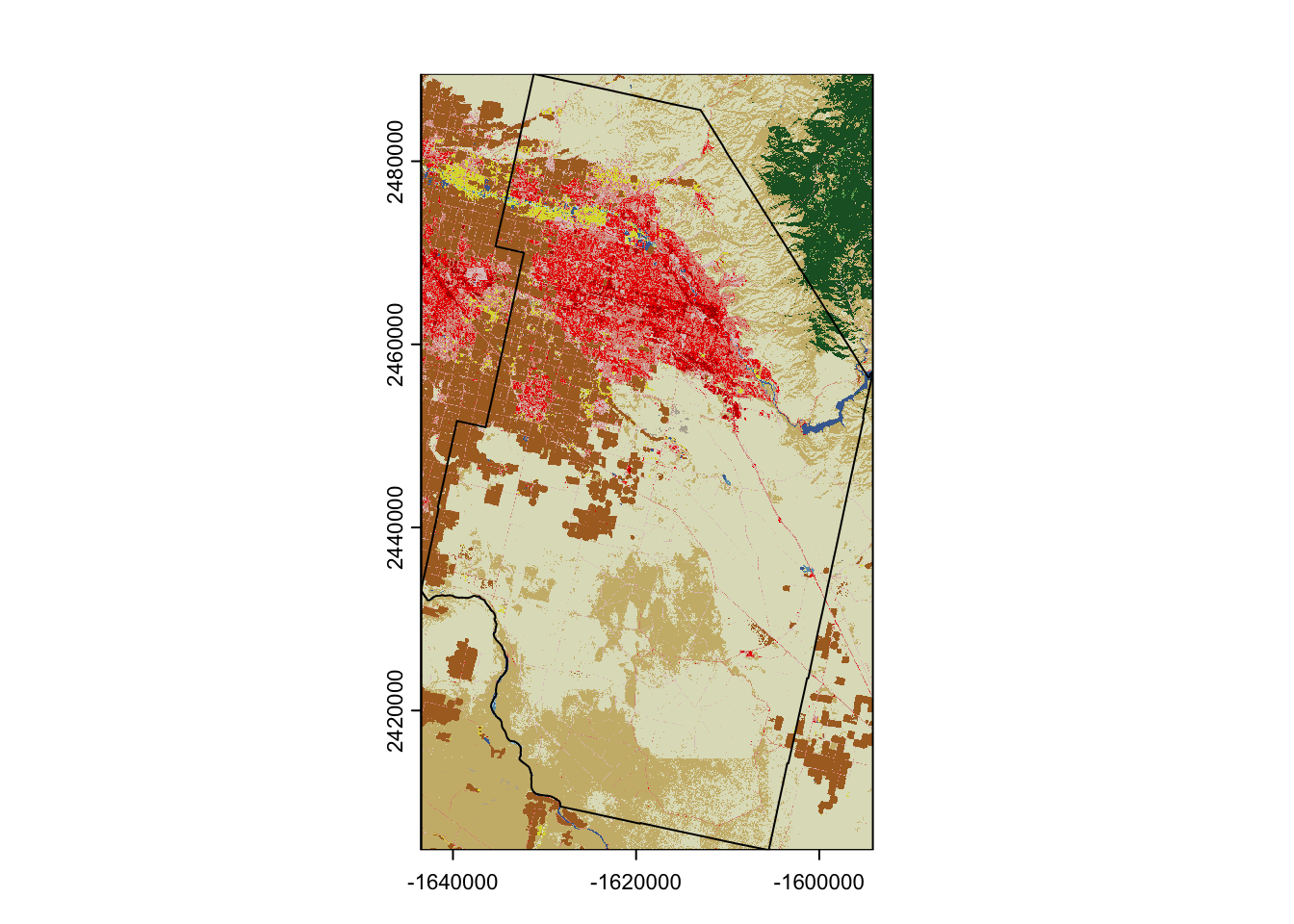
ada_NLCD <- terra::rast("https://dmsdata.cr.usgs.gov/geoserver/mrlc_Land-Cover-Native_conus_year_data/wcs?service=WCS&version=1.0.0&coverage=mrlc_Land-Cover-Native_conus_year_data:Land-Cover-Native_conus_year_data&BBOX=-1643474,2404759,-1594149,2489538&CRS=EPSG:5070&time=2020-01-01T00:00:00.000Z&format=image/geotiff&resx=30&resy=30&request=GetCoverage", vsi = FALSE)

plot(ada_NLCD)
plot(st_geometry(ada_county), add= TRUE)

The first part of this should look familiar - we’re just downloading the Ada County Boundary using the tigris package. The next part is using terra::rast to read in a file directly from the online web-service. The key part comes after the BBOX part of the link where you can plug in the correct coordinates (give an CRS) to restrict the download to something manageable. Once you’ve got it, you should be able to plot and see the different categories.

Calclulating patch metrics

The syntax for landscapemetrics is fairly straightforward with most functions starting with lsm_ followed by a letter, followed by the name of the metric. You can see the full set of patch metrics here.

Code

head(lsm_p_area(ada_NLCD))

# A tibble: 6 × 6
  layer level class    id metric   value
  <int> <chr> <int> <int> <chr>    <dbl>
1     1 patch    11     1 area     5.58 
2     1 patch    11     2 area     3.69 
3     1 patch    11     3 area     0.630
4     1 patch    11     4 area   689.   
5     1 patch    11     5 area     2.52 
6     1 patch    11     6 area     1.35

Code

head(lsm_p_shape(ada_NLCD))

# A tibble: 6 × 6
  layer level class    id metric value
  <int> <chr> <int> <int> <chr>  <dbl>
1     1 patch    11     1 shape   1.14
2     1 patch    11     2 shape   1.17
3     1 patch    11     3 shape   1.13
4     1 patch    11     4 shape  11.6 
5     1 patch    11     5 shape   1.42
6     1 patch    11     6 shape   1.16

Code

show_lsm(ada_NLCD, what = "lsm_p_area")

$layer_1

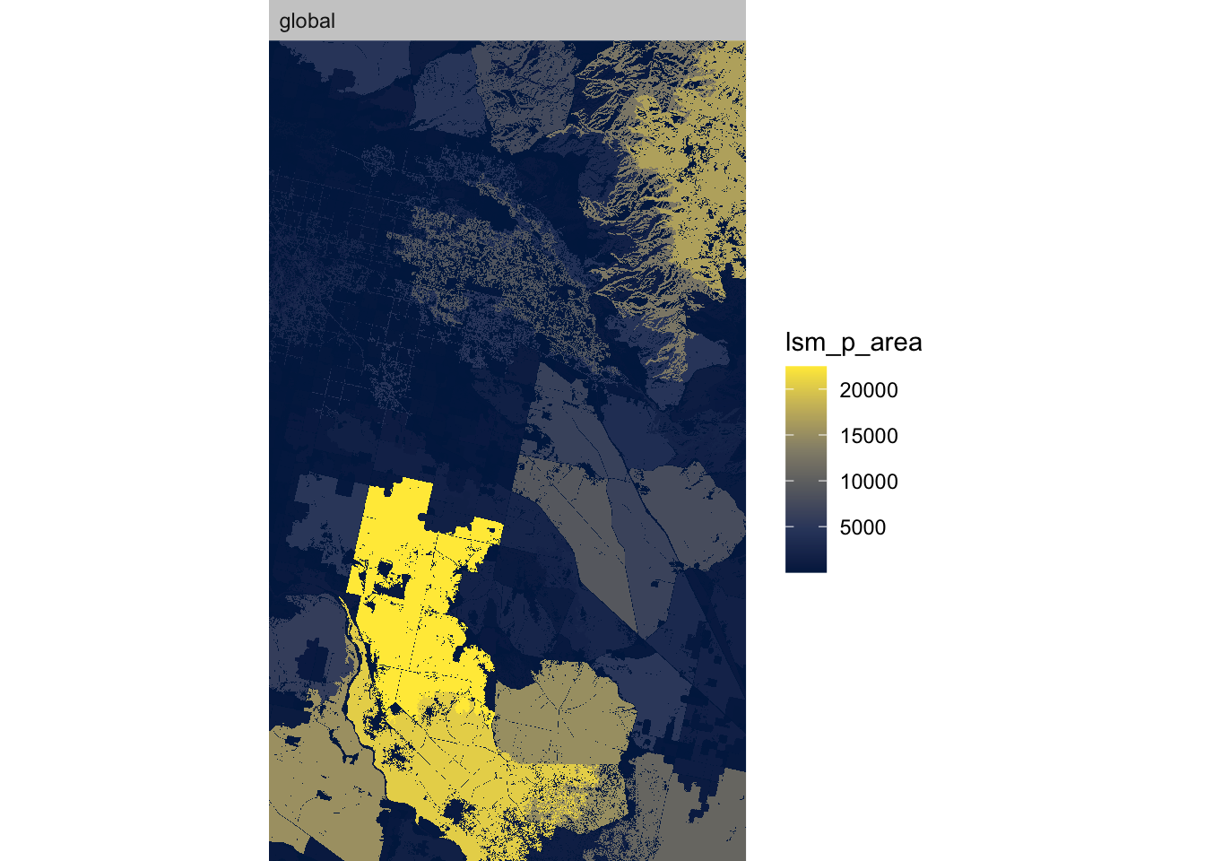
We calculate some basic patch metrics using lsm_p_METRIC, but restrict the output to the first 5 entries to make the printing easier. We also use the show_lsm function to create a map based on these patch-level metrics (this only works for patch metrics, not the class or landscape metrics). In this case, we’re interested in the patch area and shape (check out the help files for the equations). In landscapemetrics patches are defined as neighboring rasters (defined as queen or rooks case using the directions argument) that share the same category. Each of these functions estimates a measure for all of the patches in a landscape (which may be as small as 1 pixel and as large as the entire landscape).

Calculating class metrics

The full list of class metrics is here and the syntax follows the format above (but replaces the p with a c). Class metrics take all of the patches within a category and summarize them - here we calculate the percent covered, the number of patches/class, and the edge density (which is the sum of edge lengths for each patch in the class divided by the total area of the category in the landscape). These metrics can give you a sense of size and dominance of the different categories.

Code

lsm_c_pland(ada_NLCD)   # % of landscape occupied

# A tibble: 15 × 6
   layer level class    id metric     value
   <int> <chr> <int> <int> <chr>      <dbl>
 1     1 class    11    NA pland   0.527   
 2     1 class    21    NA pland   3.33    
 3     1 class    22    NA pland   7.05    
 4     1 class    23    NA pland   4.41    
 5     1 class    24    NA pland   0.677   
 6     1 class    31    NA pland   0.0639  
 7     1 class    41    NA pland   0.0828  
 8     1 class    42    NA pland   4.40    
 9     1 class    43    NA pland   0.000409
10     1 class    52    NA pland  20.8     
11     1 class    71    NA pland  44.0     
12     1 class    81    NA pland   1.28    
13     1 class    82    NA pland  13.3     
14     1 class    90    NA pland   0.0746  
15     1 class    95    NA pland   0.0706

Code

lsm_c_np(ada_NLCD)      # number of patches per class

# A tibble: 15 × 6
   layer level class    id metric value
   <int> <chr> <int> <int> <chr>  <dbl>
 1     1 class    11    NA np       382
 2     1 class    21    NA np     20237
 3     1 class    22    NA np     14793
 4     1 class    23    NA np      7012
 5     1 class    24    NA np      2720
 6     1 class    31    NA np       231
 7     1 class    41    NA np       616
 8     1 class    42    NA np       765
 9     1 class    43    NA np        15
10     1 class    52    NA np     15848
11     1 class    71    NA np      9802
12     1 class    81    NA np      2810
13     1 class    82    NA np      3886
14     1 class    90    NA np       523
15     1 class    95    NA np       429

Code

lsm_c_ed(ada_NLCD)

# A tibble: 15 × 6
   layer level class    id metric    value
   <int> <chr> <int> <int> <chr>     <dbl>
 1     1 class    11    NA ed      1.02   
 2     1 class    21    NA ed     21.9    
 3     1 class    22    NA ed     34.5    
 4     1 class    23    NA ed     18.7    
 5     1 class    24    NA ed      3.00   
 6     1 class    31    NA ed      0.265  
 7     1 class    41    NA ed      0.515  
 8     1 class    42    NA ed      3.84   
 9     1 class    43    NA ed      0.00517
10     1 class    52    NA ed     36.0    
11     1 class    71    NA ed     37.3    
12     1 class    81    NA ed      4.40   
13     1 class    82    NA ed     11.9    
14     1 class    90    NA ed      0.527  
15     1 class    95    NA ed      0.394

Calculating landscape metrics

Finally, full list of landscape metrics is here](https://r-spatialecology.github.io/landscapemetrics/reference/index.html#landscape-level-metrics). We follow the same formatting strategy to access a handful of the landscape metrics. Landscape metrics look at the juxtaposition of the different classes in your landscape. We calculate the Shannon’s Diversity Index (a measure of class evenness in the landscape) and cohesion (an estimate of contiguity between like patches).

Code

lsm_l_shdi(ada_NLCD)    # Shannon’s Diversity Index

# A tibble: 1 × 6
  layer level     class    id metric value
  <int> <chr>     <int> <int> <chr>  <dbl>
1     1 landscape    NA    NA shdi    1.67

Code

lsm_l_cohesion(ada_NLCD)

# A tibble: 1 × 6
  layer level     class    id metric   value
  <int> <chr>     <int> <int> <chr>    <dbl>
1     1 landscape    NA    NA cohesion  99.1