── Attaching core tidyverse packages ──────────────────────── tidyverse 2.0.0 ──
✔ dplyr     1.1.4     ✔ readr     2.1.5
✔ forcats   1.0.1     ✔ stringr   1.5.2
✔ ggplot2   4.0.0     ✔ tibble    3.3.0
✔ lubridate 1.9.4     ✔ tidyr     1.3.1
✔ purrr     1.1.0
── Conflicts ────────────────────────────────────────── tidyverse_conflicts() ──
✖ dplyr::filter() masks stats::filter()
✖ dplyr::lag()    masks stats::lag()
ℹ Use the conflicted package (<http://conflicted.r-lib.org/>) to force all conflicts to become errors
Code
library(terra)
terra 1.8.70

Attaching package: 'terra'

The following object is masked from 'package:tidyr':

    extract
Code
library(geodata)library(tidyterra)
Attaching package: 'tidyterra'

The following object is masked from 'package:stats':

    filter
Code
library(caret)
Loading required package: lattice

Attaching package: 'caret'

The following object is masked from 'package:purrr':

    lift
Getting Started
This exercise is going to rely on simulated data so you don’t need to join a repository. You’ll just need to get our credentials and login to a new RStudio session. We’re going to keep using the simulation so that you know what the true values are and so you can explore some of the different ways of assessing model fit.
Get the Data
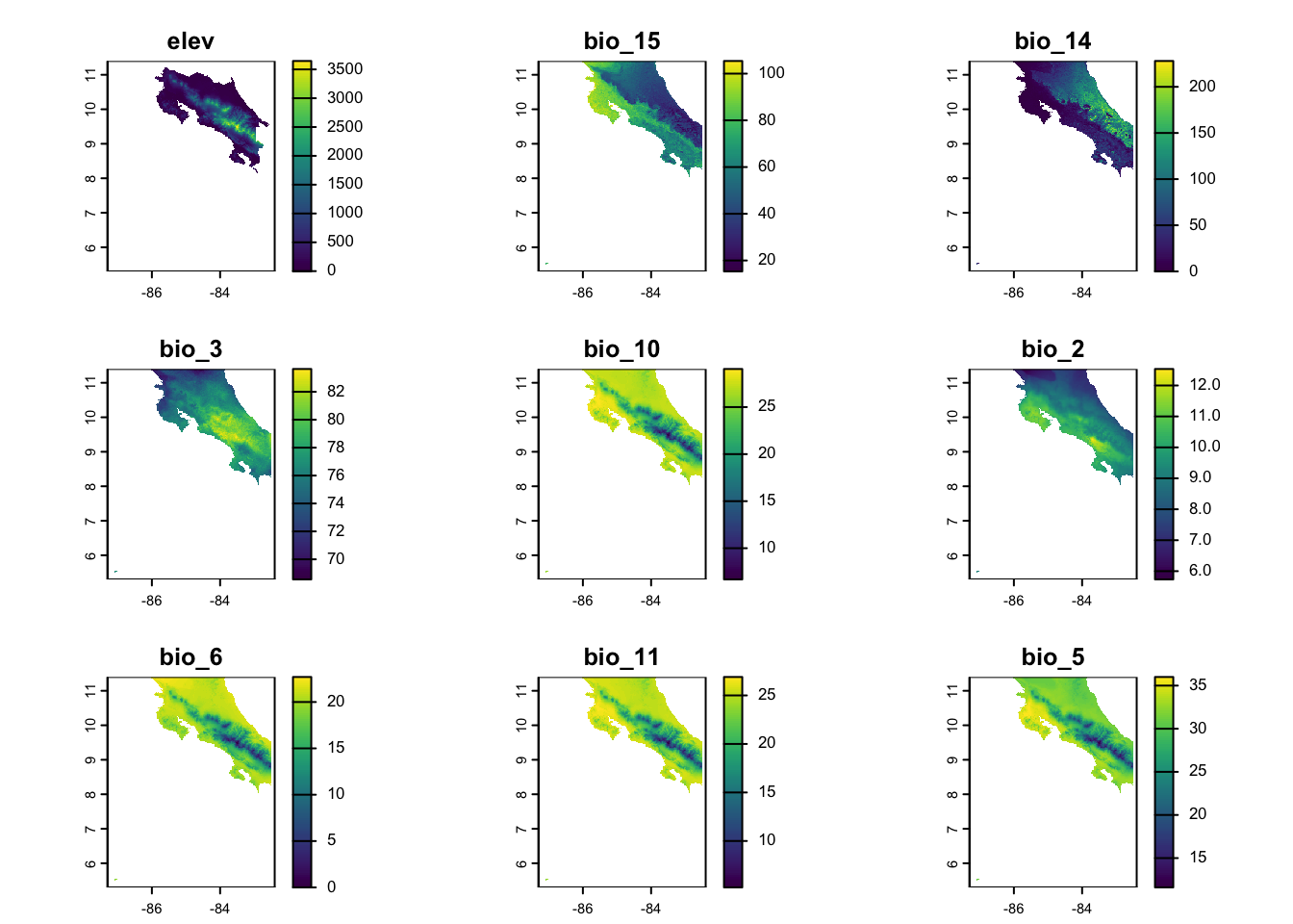
We’ll use the same approache we used before to download data for Costa Rica using the geodata package. This should (hopefully) look familiar to you.
Next we generate a sample of observations, build our dataframe (using spatSample and extract). You’ve done this before too.
Code
# Sample random locations from the study areasample_points <-spatSample(elevation, size = n_points, method ="random", na.rm =TRUE, xy =TRUE, values =FALSE)# Extract environmental values at these pointsenv_values <- terra::extract(predictors, sample_points)species_data <-tibble(x = sample_points[,1],y = sample_points[,2]) %>%bind_cols(env_values) %>%drop_na() # Remove any NA valuesspecies_data_scl <- species_data %>%mutate(across(colnames(env_values), ~as.numeric(scale(.x))))
Specify predictors
Here we’re going to simplify things a little from before. Rather than allowing for correlations between predictors, we’ll just draw a handful of \(\beta\)s from a uniform distribution. Things are already tough enough for the logistic regression given that so many of these variables are likely to be correlated (we’ll return that shortly).
Code
K <-nlyr(predictors)known_betas <-runif(n = K, min =-3, max =3)
Simulate Outcomes
Now we simulate outcomes and check to make sure we don’t end up with too many 1’s or 0’s. We use the plogis as means of converting the linear predictor to the probability scale. If you wanted to simulate different outcomes, you’d need to think through the appropriate link function.
We use the vars and form objects as a way to make this as flexible as possible (in case you end up with different predictors). In this case, it will help us later when we go to fit competing models to our initial “saturated” model.
Code
vars <- species_data_preds %>%select(colnames(env_values)) %>%names()form <-reformulate(vars, response ="presence")form
You can see from the results that we didn’t do a particularly good job of recovering the true values. Maybe more importantly, it would appear that the model didn’t do a particularly good job of converging (given the size of several of the coefficients). Remember that for logisitc regression values outside \(|\neg5, 5|\) translate to log-odds that are essentially 0 or 1, respectively.
Cohen’s Likelihood Ratio
While we can see that there are some pathologies with our model, the goal here is to decide how well this model fits the data. Because this is a logistic regression, we can’t use the standard \(R^2\) statistic. Instead we’ll look at two different Pseudo-\(R^2\) values.
To calculate Cohen’s Likelihood Ratio, we can just use elements provided to us with the model object. Namely the null.deviance and the deviance. Remember that lower values are better here (i.e., the model deviance is roughly equal that of a hypothetical perfect model). Here, we see that the value is less than 1, but larger than 0. It’s hard to know whether this is too high or not, so we’ll take a look at the Cox and Snell.
To calculate the Cox and Snell estimate, we need another model. In this case, instead of a hypotetically perfect model, we want a null model. This model tells us what we can learn without including any predictors. If our predictors have information, then the logLik of our model should be higher than that of the null. If you’re uncertain of this, experiment with running exp() for both positive and negative numbers. The larger the negative number, the smaller the decimal produced by exp and the larger the result of the equation (because we’re subtracting from 1). Here, we can see that the model isn’t terrible, but it’s not particularly good either (because we’re a ways a way from 1).
Our assessments of fit suggest the model isn’t great, but it’s not terrible either. That said, we know (from the magnitude of some of the effects and their comparison to the true values) that the model doesn’t seem to have converged particularly well. This is probably because there’s a lot of underlying correlation between the values in our predictors. We can verify that quickly using cor
The caret package gives us an easy way to identify (and potentially get rid of) correlated variables using the findCorrelation function. You’ll see that we’ve got at least 5 variables that could be dropped if we don’t want correlations to create challenges for our model. We subset our predictor vector (env_values) to remove the variables in our high_corr vector (using subset with !). Then we can fit this new subset model.
# A tibble: 10 × 5
   Parameter   True_Value Estimated Difference Pct_Error
   <chr>            <dbl>     <dbl>      <dbl>     <dbl>
 1 (Intercept)     0          0.905      0.905     Inf
 2 elev           -1.10       1.22       2.32     -212.
 3 bio_15          2.69      NA         NA          NA
 4 bio_14         -0.0585    33.1       33.1    -56652.
 5 bio_3           2.84       0.428     -2.41      -84.9
 6 bio_10          2.08      NA         NA          NA
 7 bio_2           2.88       1.63      -1.24      -43.2
 8 bio_6          -2.32      NA         NA          NA
 9 bio_11         -1.12      NA         NA          NA
10 bio_5           2.67      NA         NA          NA
Assessing Fit
Now, we know this model is not properly specified (because our simulation used all the variables), but maybe the fit statistics will help us figure out which model we might want to use (if any). We’ll calculate the Likelihood Ratio and the Cox and Snell statistic.
Unfortunately, this doesn’t help us much as the Likelihood Ratio is lower (so better than the full model), but so is the Cox and Snell (so worse than the full model).
Comparing Our Models
We can tell from this quick run through, that none of the models fit the data particularly well. But maybe we’d like to know which one does the best job. We can do that using the AIC function and providing all of the models we’d like to compare.
Based on this, it would appear that the full model has the best theoretical predictive qualities. That is the log likelihood for the full model is substantially larger than the other two models. Moreover, it’s large enough to overcome the penalty for having twice as many predictors. That said, the model didn’t converge so we might interpret these results cautiously.
Compare Model Implications
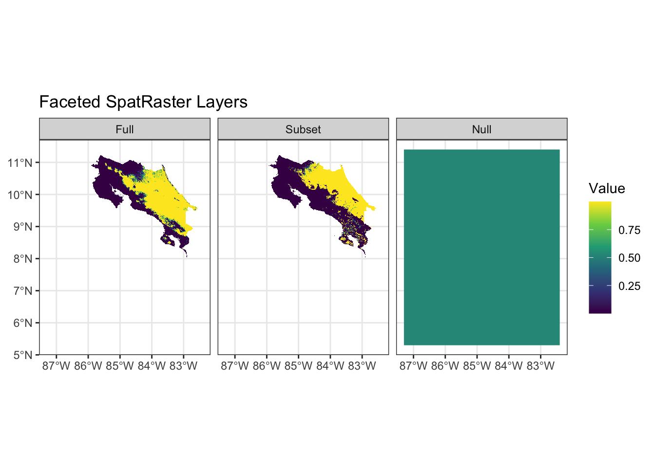
Our various tests have been pretty ambiguous - there’s no clear “best choice” for which we might use. One last check we might do, is to examine the implications of predictions from the models (as this where instability will become the most obvious). We can do that easily using the predict functions included with terra.
The plots help clarify two important things: 1) the predictions from the intercept-only model are (as expected) constant and relatively high (considering there’s no extra info in the model) and 2) the saturated model imposes a complete separation between presences and absences which indicates that we’ve perfectly separated the data generating process (unlikely). The results from the subset model seem the most plausible despite some of the diagnostics suggesting it was worse than the full model.
Take Aways
The key things I want you to remember are: 1) single tests or diagnostics are (almost) never enough 2) Each step of this process is (differently) sensitive to violations of assumptions 3) Fully interogating a model is an interative process
Source Code
---title: "Spatial Predictions and Model Assesment"---```{r}library(tidyverse)library(terra)library(geodata)library(tidyterra)library(caret)```## Getting Started This exercise is going to rely on simulated data so you don't need to join a repository. You'll just need to [get our credentials](https://rstudio.aws.boisestate.edu/) and login to a [new RStudio session](https://rstudio.apps.aws.boisestate.edu/). We're going to keep using the simulation so that you know what the true values are and so you can explore some of the different ways of assessing model fit.## Get the DataWe'll use the same approache we used before to download data for Costa Rica using the `geodata` package. This should (hopefully) look familiar to you.```{r}set.seed(123)n_points <-1000elevation <- geodata::elevation_30s(country ="CRI", path =tempdir())climate <- geodata::worldclim_country(country ="CRI", var ="bio", res =0.5, path =tempdir())names(climate) <-str_extract(names(climate), "bio_\\d+")names(elevation) <-"elev"climate_df <-as.data.frame(climate, na.rm=TRUE)climate_subset <- climate[[sample(1:nlyr(climate),size =8)]]climate_aligned <-resample(climate_subset, elevation)# Stack the predictorspredictors <-c(elevation, climate_aligned)plot(predictors)```## Generate a sampleNext we generate a sample of observations, build our dataframe (using `spatSample` and `extract`). You've done this before too.```{r}# Sample random locations from the study areasample_points <-spatSample(elevation, size = n_points, method ="random", na.rm =TRUE, xy =TRUE, values =FALSE)# Extract environmental values at these pointsenv_values <- terra::extract(predictors, sample_points)species_data <-tibble(x = sample_points[,1],y = sample_points[,2]) %>%bind_cols(env_values) %>%drop_na() # Remove any NA valuesspecies_data_scl <- species_data %>%mutate(across(colnames(env_values), ~as.numeric(scale(.x))))```## Specify predictorsHere we're going to simplify things a little from before. Rather than allowing for correlations between predictors, we'll just draw a handful of $\beta$s from a uniform distribution. Things are already tough enough for the logistic regression given that so many of these variables are likely to be correlated (we'll return that shortly).```{r}K <-nlyr(predictors)known_betas <-runif(n = K, min =-3, max =3)```## Simulate OutcomesNow we simulate outcomes and check to make sure we don't end up with too many 1's or 0's. We use the `plogis` as means of converting the linear predictor to the probability scale. If you wanted to simulate different outcomes, you'd need to think through the appropriate link function.```{r}species_data_preds <- species_data_scl %>%mutate(across(all_of(colnames(env_values)),~ .x * known_betas[which(colnames(env_values) ==cur_column())] ) ) %>%mutate(. , linpred =rowSums(across(all_of(colnames(env_values)))),prob =plogis(1+ linpred),presence =rbinom(n(), size =1, prob = prob)) # Check the prevalencespecies_data_preds %>%summarize(prevalence =mean(presence),n_present =sum(presence),n_absent =sum(presence ==0) ) ```## Fit Logistic RegressionWe use the `vars` and `form` objects as a way to make this as flexible as possible (in case you end up with different predictors). In this case, it will help us later when we go to fit competing models to our initial "saturated" model.```{r}vars <- species_data_preds %>%select(colnames(env_values)) %>%names()form <-reformulate(vars, response ="presence")formmodel <-glm(form ,data = species_data_preds,family =binomial(link ="logit"))# Model summarysummary(model)# Compare estimated coefficients to true valuestibble(Parameter =c("Intercept", colnames(env_values)),True_Value =c(0, known_betas),Estimated =coef(model),Difference = Estimated - True_Value,Pct_Error = (Difference / True_Value) *100)```You can see from the results that we didn't do a particularly good job of recovering the true values. Maybe more importantly, it would appear that the model didn't do a particularly good job of converging (given the size of several of the coefficients). Remember that for logisitc regression values outside $|\neg5, 5|$ translate to log-odds that are essentially 0 or 1, respectively.## Cohen's Likelihood RatioWhile we can see that there are some pathologies with our model, the goal here is to decide how well this model fits the data. Because this is a logistic regression, we can't use the standard $R^2$ statistic. Instead we'll look at two different Pseudo-$R^2$ values. To calculate Cohen's Likelihood Ratio, we can just use elements provided to us with the model object. Namely the `null.deviance` and the `deviance`. Remember that lower values are better here (i.e., the model deviance is roughly equal that of a hypothetical perfect model). Here, we see that the value is less than 1, but larger than 0. It's hard to know whether this is too high or not, so we'll take a look at the Cox and Snell. ```{r}(model$null.deviance - model$deviance)/model$null.deviance```## Cox and SnellTo calculate the Cox and Snell estimate, we need another model. In this case, instead of a hypotetically perfect model, we want a **null** model. This model tells us what we can learn without including any predictors. If our predictors have information, then the `logLik` of our model should be higher than that of the `null`. If you're uncertain of this, experiment with running `exp()` for both positive and negative numbers. The larger the negative number, the smaller the decimal produced by `exp` and the larger the result of the equation (because we're subtracting from 1). Here, we can see that the model isn't terrible, but it's not particularly good either (because we're a ways a way from 1).```{r}model_null <-glm(presence ~1, family=binomial(link="logit"),data=species_data_preds)1-exp(2*(logLik(model_null)[1] -logLik(model)[1])/nobs(model))```## ...But There's a ProblemOur assessments of fit suggest the model isn't great, but it's not terrible either. That said, we know (from the magnitude of some of the effects and their comparison to the true values) that the model doesn't seem to have converged particularly well. This is probably because there's a lot of underlying correlation between the values in our predictors. We can verify that quickly using `cor````{r}cor(env_values)```### Removing correlated variables The `caret` package gives us an easy way to identify (and potentially get rid of) correlated variables using the `findCorrelation` function. You'll see that we've got at least 5 variables that could be dropped if we don't want correlations to create challenges for our model. We subset our predictor vector (`env_values`) to remove the variables in our `high_corr` vector (using `subset` with `!`). Then we can fit this new subset model.```{r}cormat <-cor(species_data_preds[,colnames(env_values)], use ="pairwise.complete.obs")high_corr <-findCorrelation(cormat, cutoff =0.7, names=TRUE)sub_vars <-subset(colnames(env_values), !(colnames(env_values) %in% high_corr))vars_sub <- species_data_preds %>%select(all_of(sub_vars)) %>%names()form_sub <-reformulate(vars_sub, response ="presence")form_submodel_sub <-glm(form_sub ,data = species_data_preds,family =binomial(link ="logit"))# Model summarysummary(model_sub)# Compare estimated coefficients to true valuesresults_sub <-tibble(Parameter =c("(Intercept)", colnames(env_values)),True_Value =c(0, known_betas)) results_sub$Estimated <-coef(model_sub)[results_sub$Parameter] results_sub %>%mutate(Difference = Estimated - True_Value,Pct_Error = (Difference / True_Value) *100)```## Assessing FitNow, we know this model is not properly specified (because our simulation used all the variables), but maybe the fit statistics will help us figure out which model we might want to use (if any). We'll calculate the Likelihood Ratio and the Cox and Snell statistic. ```{r}(model_sub$null.deviance - model_sub$deviance)/model_sub$null.deviance1-exp(2*(logLik(model_null)[1] -logLik(model_sub)[1])/nobs(model_sub))```Unfortunately, this doesn't help us much as the Likelihood Ratio is lower (so better than the full model), but so is the Cox and Snell (so worse than the full model). ## Comparing Our ModelsWe can tell from this quick run through, that none of the models fit the data particularly well. But maybe we'd like to know which one does the best job. We can do that using the `AIC` function and providing all of the models we'd like to compare.```{r}AIC(model, model_sub, model_null)```Based on this, it would appear that the full model has the best theoretical predictive qualities. That is the log likelihood for the full model is substantially larger than the other two models. Moreover, it's large enough to overcome the penalty for having twice as many predictors. That said, the model didn't converge so we might interpret these results cautiously.## Compare Model ImplicationsOur various tests have been pretty ambiguous - there's no clear "best choice" for which we might use. One last check we might do, is to examine the implications of predictions from the models (as this where instability will become the most obvious). We can do that easily using the `predict` functions included with `terra`. ```{r}scale_stack <-scale(predictors)pred_model <- terra::predict(object = scale_stack,model = model,type ="response")pred_sub <- terra::predict(object = scale_stack,model = model_sub,type ="response")pred_null <- terra::predict(object = scale_stack,model = model_null,type ="response")pred_stacks <-c(pred_model, pred_sub, pred_null)names(pred_stacks) <-c("Full", "Subset", "Null")ggplot() +geom_spatraster(data = pred_stacks) +facet_wrap(~lyr) +scale_fill_viridis_c(na.value ="transparent") +labs(title ="Faceted SpatRaster Layers", fill ="Value") +theme_bw()```The plots help clarify two important things: 1) the predictions from the intercept-only model are (as expected) constant and relatively high (considering there's no extra info in the model) and 2) the saturated model imposes a complete separation between presences and absences which indicates that we've perfectly separated the data generating process (unlikely). The results from the subset model seem the most plausible despite some of the diagnostics suggesting it was worse than the full model.## Take AwaysThe key things I want you to remember are:1) single tests or diagnostics are (almost) never enough2) Each step of this process is (differently) sensitive to violations of assumptions3) Fully interogating a model is an interative process