Assignment 01 Solutions

For Your Revision

In order to facilitate you thinking about your assignment, I’m providing how I would approach each of the tasks listed in the assignment. This should allow you to go in and identify places where a) your code runs but produces a different outcome, b) your code is different but produces the same outcome, and c) your code doesn’t run because you were missing something. There is something to learn from each of these outcomes. When you revise your code, I don’t want you to just copy what I’ve done, think about your underlying logic and compare it to what I’ve written. You don’t have to agree with me (or even use the syntax I used), you just have to understand what you did!! If there are places where you are feeling fuzzy or want more explanation, note them on your revised assignment and I’ll try to address it in class or in my response to your assignment.

library(tidyverse)
── Attaching core tidyverse packages ──────────────────────── tidyverse 2.0.0 ──
✔ dplyr     1.1.4     ✔ readr     2.1.5
✔ forcats   1.0.1     ✔ stringr   1.5.2
✔ ggplot2   4.0.0     ✔ tibble    3.3.0
✔ lubridate 1.9.4     ✔ tidyr     1.3.1
✔ purrr     1.1.0     
── Conflicts ────────────────────────────────────────── tidyverse_conflicts() ──
✖ dplyr::filter() masks stats::filter()
✖ dplyr::lag()    masks stats::lag()
ℹ Use the conflicted package (<http://conflicted.r-lib.org/>) to force all conflicts to become errors

Part I: Importing and inspecting

Tasks:

  1. Use list.files, read_, and map to load the data into R.
file_names <- list.files("/Users/mattwilliamson/Websites/isdr_assignments/assignment_01_org/data/original/", pattern = ".csv", full.names = TRUE)

state_abbr <- file_names %>%
  basename() %>% 
  str_extract("(?<=_)[:alpha:]+(?=\\.csv$)")

purple_air_list <- file_names %>% 
  map(., read_csv) %>% 
  set_names(state_abbr)
Rows: 435 Columns: 9
── Column specification ────────────────────────────────────────────────────────
Delimiter: ","
chr  (1): name
dbl  (6): id, humidity, temperature, pm2.5_atm, pm2.5_cf_1, uptime
dttm (2): time_stamp, date_up

ℹ Use `spec()` to retrieve the full column specification for this data.
ℹ Specify the column types or set `show_col_types = FALSE` to quiet this message.
Rows: 327 Columns: 9
── Column specification ────────────────────────────────────────────────────────
Delimiter: ","
chr  (1): name
dbl  (6): id, humidity, temperature, pm2.5_atm, pm2.5_cf_1, uptime
dttm (2): time_stamp, date_up

ℹ Use `spec()` to retrieve the full column specification for this data.
ℹ Specify the column types or set `show_col_types = FALSE` to quiet this message.
Rows: 563 Columns: 9
── Column specification ────────────────────────────────────────────────────────
Delimiter: ","
chr  (1): name
dbl  (6): id, humidity, temperature, pm2.5_atm, pm2.5_cf_1, uptime
dttm (2): time_stamp, date_up

ℹ Use `spec()` to retrieve the full column specification for this data.
ℹ Specify the column types or set `show_col_types = FALSE` to quiet this message.
Rows: 603 Columns: 9
── Column specification ────────────────────────────────────────────────────────
Delimiter: ","
chr  (1): name
dbl  (6): id, humidity, temperature, pm2.5_atm, pm2.5_cf_1, uptime
dttm (2): time_stamp, date_up

ℹ Use `spec()` to retrieve the full column specification for this data.
ℹ Specify the column types or set `show_col_types = FALSE` to quiet this message.
names(purple_air_list)
[1] "ID" "MT" "OR" "WA"

This one should be pretty straightforward. The only tricky bits are that I set the pattern argument to ".csv" to make sure that I’m getting the right files for read_csv (which in this case is less important because that’s all that’s in the folder). I also set the full.names argument to TRUE to avoid issues when I render this file. The second tricky bit is getting the geography (i.e., state) from the data. To do this, i have to use a bit of regex wizardry in the str_exract function. The "(?<=_)[:alpha:]+(?=\\.csv$)" translates to “take any and all letters that appear after the last _ and before .csv appears at the end of the basename(). This is a generic way to extract any text between an underscore and a file extension so I show you it here, but with 4 files you could probably do this manually.

  1. Use dim(), names(), glimpse(), and summary() to explore the datasets.
purple_air_list %>% 
  map(., dim)
$ID
[1] 435   9

$MT
[1] 327   9

$OR
[1] 563   9

$WA
[1] 603   9
purple_air_list %>% 
  walk(., glimpse)
Rows: 435
Columns: 9
$ id          <dbl> 7494, 7494, 7494, 7494, 7494, 7494, 7494, 7494, 7494, 7494…
$ time_stamp  <dttm> 2025-04-01, 2024-04-01, 2021-03-01, 2022-11-01, 2022-07-0…
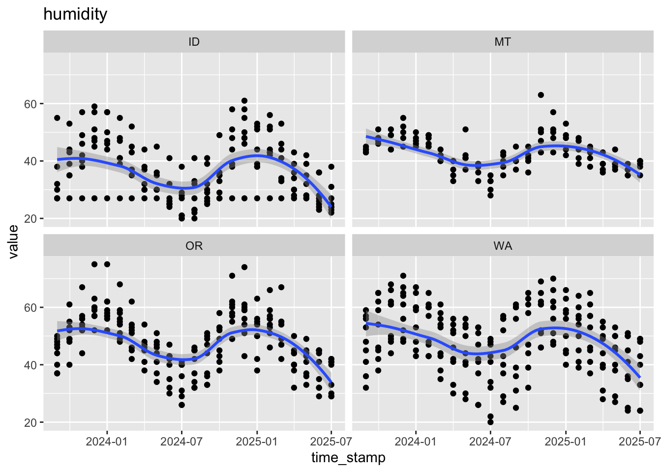
$ humidity    <dbl> 30, 30, 30, 41, 20, 27, 21, 30, 35, 29, 32, 24, 33, 46, 30…
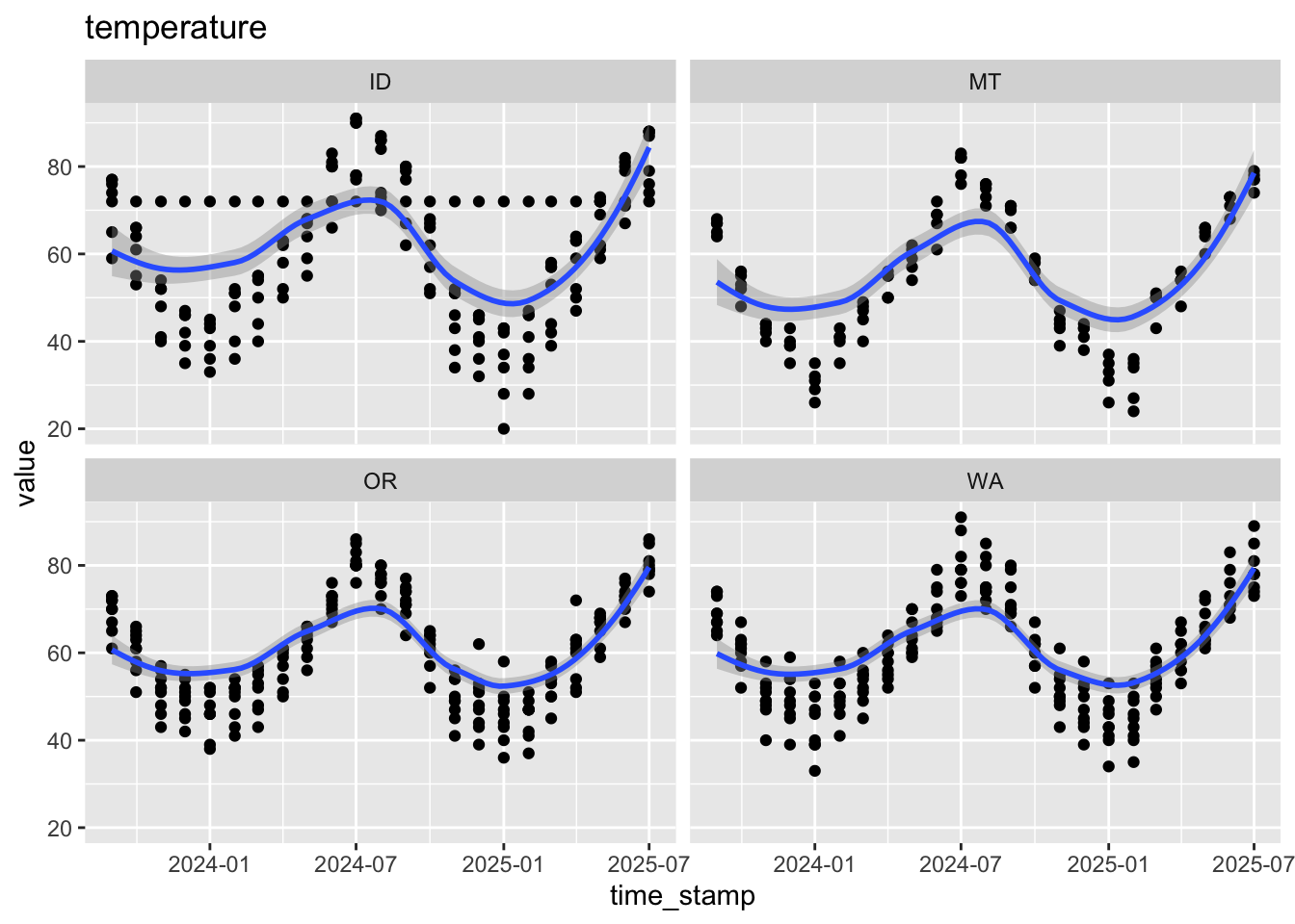
$ temperature <dbl> 63, 63, 56, 45, 91, 83, 91, 76, 66, 79, 57, 82, 66, 45, 86…
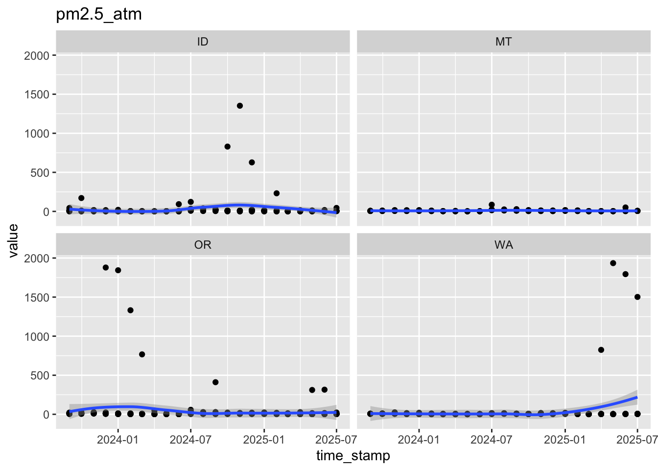
$ pm2.5_atm   <dbl> 3.7, 2.2, 4.7, 18.8, 7.3, 27.4, 30.0, 23.1, 1.8, 20.1, 3.9…
$ pm2.5_cf_1  <dbl> 3.7, 2.2, 4.8, 20.2, 7.5, 33.8, 38.3, 31.3, 1.8, 25.6, 4.0…
$ name        <chr> "MesaVista", "MesaVista", "MesaVista", "MesaVista", "MesaV…
$ date_up     <dttm> 2018-02-10 03:05:11, 2018-02-10 03:05:11, 2018-02-10 03:0…
$ uptime      <dbl> 42661, 42661, 42661, 42661, 42661, 42661, 42661, 42661, 42…
Rows: 327
Columns: 9
$ id          <dbl> 36673, 36673, 36673, 36673, 36673, 36673, 36673, 36673, 36…
$ time_stamp  <dttm> 2022-08-01, 2020-05-01, 2024-01-01, 2021-08-01, 2021-03-0…
$ humidity    <dbl> 37, 45, 47, 46, 40, 48, 49, 41, 47, 48, 39, 40, 47, 44, 50…
$ temperature <dbl> 77, 60, 32, 71, 46, 39, 42, 45, 40, 35, 64, 52, 55, 59, 38…
$ pm2.5_atm   <dbl> 12.1, 2.8, 16.4, 29.5, 98.9, 9.4, 10.7, 6.4, 7.3, 8.3, 4.2…
$ pm2.5_cf_1  <dbl> 12.8, 3.0, 17.2, 37.1, 145.6, 9.9, 11.5, 6.7, 7.7, 8.9, 4.…
$ name        <chr> "419 S. 4th St", "419 S. 4th St", "419 S. 4th St", "419 S.…
$ date_up     <dttm> 2019-08-02 19:28:01, 2019-08-02 19:28:01, 2019-08-02 19:2…
$ uptime      <dbl> 15585, 15585, 15585, 15585, 15585, 15585, 15585, 15585, 15…
Rows: 563
Columns: 9
$ id          <dbl> 9810, 9810, 9810, 9810, 9810, 9810, 9810, 9810, 9810, 9810…
$ time_stamp  <dttm> 2020-11-01, 2021-05-01, 2020-05-01, 2023-12-01, 2020-09-0…
$ humidity    <dbl> 45, 32, 38, 52, 30, 43, 22, 49, 35, 38, 38, 51, 25, 46, 37…
$ temperature <dbl> 46, 63, 62, 46, 72, 47, 89, 45, 69, 54, 55, 44, 55, 41, 48…
$ pm2.5_atm   <dbl> 23.1, 3.9, 4.5, 23.6, 56.1, 12.6, 31.9, 13.0, 2.7, 6.2, 25…
$ pm2.5_cf_1  <dbl> 27.4, 4.3, 4.6, 28.3, 79.9, 13.7, 40.5, 14.2, 2.7, 6.3, 30…
$ name        <chr> "PSU STAR LAB KFP", "PSU STAR LAB KFP", "PSU STAR LAB KFP"…
$ date_up     <dttm> 2018-04-11 23:19:19, 2018-04-11 23:19:19, 2018-04-11 23:1…
$ uptime      <dbl> 22520, 22520, 22520, 22520, 22520, 22520, 22520, 22520, 22…
Rows: 603
Columns: 9
$ id          <dbl> 18161, 18161, 18161, 18161, 18161, 18161, 18161, 18161, 18…
$ time_stamp  <dttm> 2020-08-01, 2023-01-01, 2022-03-01, 2024-01-01, 2023-10-0…
$ humidity    <dbl> 47, 57, 58, 59, 59, 50, 61, 61, 54, 48, 42, 61, 60, 50, 51…
$ temperature <dbl> 75, 52, 55, 50, 62, 52, 56, 54, 54, 72, 79, 47, 52, 72, 55…
$ pm2.5_atm   <dbl> 5.7, 2.8, 4.2, 3.5, 6.4, 3.2, 2.7, 4.6, 3.1, 16.0, 7.5, 4.…
$ pm2.5_cf_1  <dbl> 5.7, 2.8, 4.4, 3.6, 6.4, 3.3, 2.8, 4.7, 3.2, 18.3, 8.0, 4.…
$ name        <chr> "Issaquah Highlands", "Issaquah Highlands", "Issaquah High…
$ date_up     <dttm> 2018-10-29 22:26:57, 2018-10-29 22:26:57, 2018-10-29 22:2…
$ uptime      <dbl> 13394, 13394, 13394, 13394, 13394, 13394, 13394, 13394, 13…
purple_air_list %>% 
  map(., \(x) summary(x))
$ID
       id          time_stamp                     humidity      temperature   
 Min.   : 7494   Min.   :2020-01-01 00:00:00   Min.   :18.00   Min.   :20.00  
 1st Qu.:10906   1st Qu.:2021-07-16 12:00:00   1st Qu.:27.00   1st Qu.:47.00  
 Median :27287   Median :2023-02-01 00:00:00   Median :34.00   Median :63.00  
 Mean   :23317   Mean   :2022-12-13 05:17:47   Mean   :35.44   Mean   :61.88  
 3rd Qu.:36707   3rd Qu.:2024-06-01 00:00:00   3rd Qu.:42.50   3rd Qu.:74.50  
 Max.   :40715   Max.   :2025-07-01 00:00:00   Max.   :82.00   Max.   :93.00  
   pm2.5_atm         pm2.5_cf_1         name          
 Min.   :   0.00   Min.   :   0.0   Length:435        
 1st Qu.:   2.55   1st Qu.:   2.6   Class :character  
 Median :   5.40   Median :   5.6   Mode  :character  
 Mean   :  21.34   Mean   :  29.1                     
 3rd Qu.:  11.90   3rd Qu.:  12.7                     
 Max.   :1352.50   Max.   :2008.4                     
    date_up                        uptime     
 Min.   :2018-02-10 03:05:11   Min.   : 1114  
 1st Qu.:2018-05-16 21:09:00   1st Qu.: 2210  
 Median :2019-02-20 18:49:10   Median :16424  
 Mean   :2018-12-19 01:32:17   Mean   :22545  
 3rd Qu.:2019-08-06 20:56:44   3rd Qu.:42661  
 Max.   :2019-11-05 18:27:41   Max.   :51249  

$MT
       id          time_stamp                     humidity      temperature   
 Min.   : 2851   Min.   :2020-01-01 00:00:00   Min.   :26.00   Min.   :24.00  
 1st Qu.:13975   1st Qu.:2021-06-16 00:00:00   1st Qu.:39.00   1st Qu.:41.00  
 Median :28423   Median :2022-11-01 00:00:00   Median :42.00   Median :52.00  
 Mean   :22563   Mean   :2022-10-16 10:16:30   Mean   :42.17   Mean   :53.99  
 3rd Qu.:31595   3rd Qu.:2024-03-01 00:00:00   3rd Qu.:46.00   3rd Qu.:68.00  
 Max.   :36673   Max.   :2025-07-01 00:00:00   Max.   :63.00   Max.   :84.00  
   pm2.5_atm         pm2.5_cf_1          name          
 Min.   :   1.40   Min.   :   1.50   Length:327        
 1st Qu.:   3.55   1st Qu.:   3.65   Class :character  
 Median :   6.30   Median :   6.50   Mode  :character  
 Mean   :  15.23   Mean   :  19.52                     
 3rd Qu.:  11.45   3rd Qu.:  12.40                     
 Max.   :1213.90   Max.   :1819.60                     
    date_up                        uptime     
 Min.   :2017-08-14 20:26:35   Min.   : 5798  
 1st Qu.:2018-08-02 22:50:59   1st Qu.: 8587  
 Median :2019-03-11 20:13:09   Median :15362  
 Mean   :2018-11-10 07:57:48   Mean   :16822  
 3rd Qu.:2019-05-08 17:02:54   3rd Qu.:15585  
 Max.   :2019-08-02 19:28:01   Max.   :37460  

$OR
       id          time_stamp                     humidity      temperature   
 Min.   : 3192   Min.   :2020-01-01 00:00:00   Min.   :22.00   Min.   :34.00  
 1st Qu.:14923   1st Qu.:2021-05-01 00:00:00   1st Qu.:40.00   1st Qu.:49.00  
 Median :24241   Median :2022-11-01 00:00:00   Median :46.00   Median :59.00  
 Mean   :22478   Mean   :2022-10-19 10:41:59   Mean   :46.65   Mean   :60.25  
 3rd Qu.:31141   3rd Qu.:2024-03-01 00:00:00   3rd Qu.:54.00   3rd Qu.:72.00  
 Max.   :35383   Max.   :2025-07-01 00:00:00   Max.   :75.00   Max.   :93.00  
   pm2.5_atm         pm2.5_cf_1          name          
 Min.   :   0.80   Min.   :   0.80   Length:563        
 1st Qu.:   4.00   1st Qu.:   4.10   Class :character  
 Median :   7.10   Median :   7.20   Mode  :character  
 Mean   :  35.14   Mean   :  49.23                     
 3rd Qu.:  13.25   3rd Qu.:  14.90                     
 Max.   :1878.60   Max.   :2816.70                     
    date_up                        uptime     
 Min.   :2017-09-08 19:19:21   Min.   :  394  
 1st Qu.:2018-09-04 20:07:59   1st Qu.: 9047  
 Median :2019-01-09 21:26:33   Median :11514  
 Mean   :2018-11-23 19:08:32   Mean   :18393  
 3rd Qu.:2019-05-01 16:16:43   3rd Qu.:22520  
 Max.   :2019-07-18 20:12:09   Max.   :46517  

$WA
       id          time_stamp                     humidity      temperature
 Min.   : 2651   Min.   :2020-01-01 00:00:00   Min.   :19.00   Min.   :29  
 1st Qu.:14981   1st Qu.:2021-05-01 00:00:00   1st Qu.:41.00   1st Qu.:49  
 Median :18161   Median :2022-10-01 00:00:00   Median :50.00   Median :59  
 Mean   :22431   Mean   :2022-10-01 03:56:25   Mean   :48.28   Mean   :60  
 3rd Qu.:36463   3rd Qu.:2024-03-01 00:00:00   3rd Qu.:56.00   3rd Qu.:71  
 Max.   :42073   Max.   :2025-07-01 00:00:00   Max.   :71.00   Max.   :92  
   pm2.5_atm         pm2.5_cf_1          name          
 Min.   :   0.60   Min.   :   0.60   Length:603        
 1st Qu.:   3.40   1st Qu.:   3.50   Class :character  
 Median :   5.20   Median :   5.30   Mode  :character  
 Mean   :  18.24   Mean   :  24.51                     
 3rd Qu.:   8.50   3rd Qu.:   8.85                     
 Max.   :1934.70   Max.   :2902.10                     
    date_up                        uptime     
 Min.   :2017-08-08 18:14:55   Min.   : 1242  
 1st Qu.:2018-09-04 20:17:30   1st Qu.: 4217  
 Median :2018-10-29 22:26:57   Median : 6789  
 Mean   :2018-12-08 04:09:13   Mean   :10275  
 3rd Qu.:2019-08-01 19:33:48   3rd Qu.:10340  
 Max.   :2019-11-21 18:34:00   Max.   :39183  

This one should also be pretty straightforward. One thing you’ll notice is that I used walk for glimpse, but had to use map for the other two. This is because glimpse is part of the tidyverse and so was designed to be called in a pipeline where the primary interest is not in saving the result to an object, but rather to get the side effect (which is what walk is good for). The other two functions (dim and summary) are from base R and so they behave a little differently.I

  1. Identify at least two potential data quality issues (e.g., missing values, inconsistent categories, unrealistic ranges). Explain why you think these data might be incorrect and how you might go about verifying them.

To me, the biggest risks here are the fact that the id column has been treated as numeric when it’s almost certainly supposed to be a character. Beyond that, the Max values for the pm2.5 columns are quite a bit larger than the mean or median suggesting they may be spurious. However, we imagine that these values should “spike” when there’s a fire, so we might check to see when those observations occur.

purple_air_list %>% 
  map(.,\(x) slice_max(x,
                       order_by = pm2.5_atm,
                       n=3))
$ID
# A tibble: 3 × 9
     id time_stamp          humidity temperature pm2.5_atm pm2.5_cf_1 name      
  <dbl> <dttm>                 <dbl>       <dbl>     <dbl>      <dbl> <chr>     
1 10906 2024-11-01 00:00:00       38          51     1352.      2008. NussHaus  
2 40715 2020-09-01 00:00:00       29          65     1205.      1805. Fish Have…
3 10906 2024-10-01 00:00:00       27          68      830.      1221. NussHaus  
# ℹ 2 more variables: date_up <dttm>, uptime <dbl>

$MT
# A tibble: 3 × 9
     id time_stamp          humidity temperature pm2.5_atm pm2.5_cf_1 name      
  <dbl> <dttm>                 <dbl>       <dbl>     <dbl>      <dbl> <chr>     
1 36673 2021-04-01 00:00:00       36          53     1214.      1820. 419 S. 4t…
2 36673 2021-05-01 00:00:00       40          60      335.       502. 419 S. 4t…
3 36673 2021-06-01 00:00:00       38          74      210.       313. 419 S. 4t…
# ℹ 2 more variables: date_up <dttm>, uptime <dbl>

$OR
# A tibble: 3 × 9
     id time_stamp          humidity temperature pm2.5_atm pm2.5_cf_1 name      
  <dbl> <dttm>                 <dbl>       <dbl>     <dbl>      <dbl> <chr>     
1 22983 2023-12-01 00:00:00       60          52     1879.      2817. Concordia 
2 22983 2024-01-01 00:00:00       59          46     1844.      2765. Concordia 
3  3192 2020-09-01 00:00:00       34          69     1830.      2743. Redmond H…
# ℹ 2 more variables: date_up <dttm>, uptime <dbl>

$WA
# A tibble: 3 × 9
     id time_stamp          humidity temperature pm2.5_atm pm2.5_cf_1 name      
  <dbl> <dttm>                 <dbl>       <dbl>     <dbl>      <dbl> <chr>     
1 14115 2025-05-01 00:00:00       38          63     1935.      2902. Tumble Cr…
2 14115 2025-06-01 00:00:00       35          71     1794.      2690. Tumble Cr…
3 14115 2025-07-01 00:00:00       33          78     1502.      2252. Tumble Cr…
# ℹ 2 more variables: date_up <dttm>, uptime <dbl>

Looking at the results doesn’t give us any real reason to believe that all of these correspond with fires (because several of them happen in the winter or spring), but also don’t give us a ton of reason to suspect that they’re wrong (because within a state they correspond to relatively consistent time periods). We’ll go forward and trust that PurpleAir’s data cleaners have done a good job.

Reflection

  1. What assumptions are you making about the data? Are they a reasonable sample? What biases that might exist? Do the potential errors you’ve spotted impact your analysis?

This one is mostly for you, but my initial thoughts are: These data come from people/places where air quality was a concern for some reason. The sensors cost money so they aren’t distributed randomly on the landscape or with respect to other socio-demgraphic data. For something as “global” as atmospheric movements of smoke, we might imagine that these finer-scale factors aren’t going to bias the broader spatial trend in smoke. But there are some pretty big “holes” in where these data exist that might make it tough to argue that. I also think the strange “max” values in the data suggest that in some places, we risk misattributing pm2.5 to fire when it might actually be caused by something else.

Part 2: Data Manipulation with tidyverse

Tasks

Use dplyr to:

  1. Combine all of the datasets into a single dataframe
pm25_df <- purple_air_list %>% 
  list_rbind(., names_to = "state")

sum(
  map_vec(
    purple_air_list, \(x) nrow(x))
    )
[1] 1928
colnames(pm25_df)
 [1] "state"       "id"          "time_stamp"  "humidity"    "temperature"
 [6] "pm2.5_atm"   "pm2.5_cf_1"  "name"        "date_up"     "uptime"     

I’ll walk through each of these steps, though can really do many of them in a single pipeline. First, I use list_rbind to collapse the lists into a single dataframe and use the names for each slot in the list as an entry into a new column called state(in class, we used bind_rows and they will both work, but the syntax for list_rbind is a little cleaner in the case where we want each name to be a part of the data). I can do this because all of the elements in my list have the same columns. I then perform a “sanity check” to make sure that this worked as expected by comparing the number of rows (nrow) in my resulting pm25_df object to the number of rows I get when accessing each dataframe in my list. I calculate this by using map_vec (because I want a vector with the nrow from each df in the list) and passing the result to sum. Both numbers are equal so we can move on, but if they weren’t, I’d be concerned that bind_rows had dropped some observations.

  1. Select variables relevant to the overarching research question.
pm25_df <- purple_air_list %>% 
   list_rbind(., names_to = "state") %>% 
  select(id, time_stamp, humidity, temperature, pm2.5_atm, state)

colnames(pm25_df)
[1] "id"          "time_stamp"  "humidity"    "temperature" "pm2.5_atm"  
[6] "state"      

I build on the previous pipeline by adding a simple select call for the variables we want. I keep the id and time_stamp variables because I know we’ll need them for filtering and pivoting later. Otherwise, I focus only on the columns with the information I want related to the research question.

  1. Filter the data to observations from the last 2 years and create a new column that calculates the monthly change in pm2.5 (hint: you’ll need mutate, arrange, and lag)
pm25_df <- purple_air_list %>% 
   list_rbind(., names_to = "state") %>% 
  select(id, time_stamp, humidity, temperature, pm2.5_atm, state) %>% 
  filter(time_stamp > ymd("2023-08-31")) %>% 
  mutate(
    month = floor_date(time_stamp, "month")  # round timestamps to the month
  ) %>% 
  group_by(id) %>% 
  arrange(month, .by_group = TRUE) %>%
  mutate(pm25_change = pm2.5_atm - lag(pm2.5_atm))

summary(pm25_df$pm25_change)
     Min.   1st Qu.    Median      Mean   3rd Qu.      Max.      NA's 
-1332.100    -2.550    -0.100     2.092     1.800  1867.100        31 
length(unique(pm25_df$id))
[1] 31

Building on our pipeline from before, I add a filter call. The time_stamp variable has a dttm class which means that it encodes dates (and times) in a particular way (in this case as a POSIXct object). I use the lubridate::ymd function to convert a string ("08-31-2023") to a year-month-date object (which is how the dates in time_stamp are formatted) and filter for all observations before that date. Then comes the tricky bit, I use floor_date (a function which rounds down to the nearest month) to create a new variable, month, inside of a mutate call. I then group_by each id (to keep the sensors separate) and arrange by month within each group (.by_group=TRUE). This sorts the data from the earliest month for each id. Finally, I calculate the change in pm2.5 by using the lag function to subtract the previous row’s value from the current row’s value. I expect NAs in this calculation for the first observation in each id, because there’s nothing to subtract. I double check this by comparing the results of the summary and length calls for each data set. Note that there are other ways to do this, but this is the most literal translation of the instructions to code.

  1. Group the data by year and state to calculate the annual mean and standard deviation of all numeric variables for each state.
pm25_df_grp <- pm25_df %>%  
  group_by(state, year = year(time_stamp)) %>% 
  select(!id) %>% 
  summarise(across(
      where(is.numeric),
      list(mean = ~mean(.x, na.rm = TRUE),
           sd   = ~sd(.x, na.rm = TRUE)),
      .names = "{.col}_{.fn}"
    ),
    .groups = "drop"
  )

I took the dataframe from our previous step and passed it to group_by using lubridate::year to create a new grouping variable called year. Then, because I want to create a new value based on the grouped data, I use summarise with some helpers. The across(where()) combination says that I want to apply the summary function across all the columns where is.numeric==TRUE (the across and where functions are dplyr::select helpers). Because I want to apply two different summaries across the selected columns and be able to drop NA values, I have to provide those functions inside a list. The list contains the functions (applied to the columns selected by the helpers) and any additional arguments to the functions (like na.rm=TRUE). Finally, I provide the .names= argument to tell across what I want the names to be. You’ll notice that I used select to drop the id variable (!id means not id) because it was considered numeric when we read the data into R. I knew this would come back to haunt me!!

  1. Convert the ungrouped dataset from wide to long format.
pm25_df_long <- pm25_df %>% 
  pivot_longer(cols=c(humidity:pm2.5_atm, 
                      pm25_change), 
               names_to = "measure")

pm25_df_grp_long <- pm25_df_grp %>% 
  pivot_longer(cols = humidity_mean:pm25_change_sd, 
               names_to = "measure")

In case you were confused about which dataset I mean, I show you pivot_longer for both. The key here is that we have more than one column that uniquely identifies each observation (id and time_stamp in the original dataset, state and year in the second). I use the : to specify column a through column b for columns that are contiguous in the data. For the pm25_df data, I need to skip a few columns so I use the : in combination with the c function to put them all together. Finally, I use the names_to agrument to pivot_longer to specify what I want the new variable column to be called.

Reflection

  1. How does tidyverse syntax support transparent and reproducible analysis? You’ll notice in my explanation above, that many of my sentences are actually just narrating the exact code I wrote. This is the power of tidyverse - it translates computer language into human-readable language. The pipes combine functions such that they “read” like instructions. In addition, I am able to run all of these commands within the tidyverse making the codestyle consistent and reducing dependencies on packages that may be updated less frequently.
  2. In what ways could poor coding style or inconsistent workflows make this analysis harder for collaborators? This one’s for you!! ## Part 3: Functions and Iteration

Tasks

  1. Write a function that filters your long-format data by a variable and generates a plot of that variable through time for each state. Do this in two steps. Write the function in pseudocode in this block:
1. pass data to function
2. filter `measure` for `variable`
3. plot `value` 
4. add trend
4. facet

This is a bit of a “dealers choice” you should write this in a way that helps you focus on what you need the function to do. I wanted to think through the things I wanted on the plot - namely, the data themselves and a smoothed trendline

Then create the function in this block:

plot_through_time <- function(df, variable){
  df_filt <- df %>% 
    filter(measure == variable)
  ggplot(data = df_filt, aes(x = time_stamp, 
                             y = value)) +
    geom_point()+
    geom_smooth() +
    facet_wrap(~state) +
    ggtitle(variable)
}

I gave my function a useful, but generic name and assumed I would only need two arguments, df for the original data and variable for the measure I wanted to use. Having the data in long format helps us here as we don’t have to deal with embracing variable names. Once, we’ve got the filtering correct, it’s a matter of preference for plot elements.

  1. Create a vector of variables and use your function to generate a list of plots (using map).
plot_vars <- c("temperature", "humidity", "pm2.5_atm","pm25_change")

time_series_plots <- map(plot_vars, ~ plot_through_time(df = pm25_df_long, variable = .x))

walk(time_series_plots, print)
`geom_smooth()` using method = 'loess' and formula = 'y ~ x'

`geom_smooth()` using method = 'loess' and formula = 'y ~ x'

`geom_smooth()` using method = 'loess' and formula = 'y ~ x'

`geom_smooth()` using method = 'loess' and formula = 'y ~ x'
Warning: Removed 31 rows containing non-finite outside the scale range
(`stat_smooth()`).
Warning: Removed 31 rows containing missing values or values outside the scale range
(`geom_point()`).

Now that we’ve got our function, I’ll just pass a vector of measures (in plot_vars) to map and iterate through it. I can then use walk to pass each element in the my time_series_plots list to print to be able to see them all. The plots aren’t particularly pretty, though we do see some nice seasonal signatures in temperature and humidity and variation in the intensity of those cycles across states. The pm2.5_atm and pm25_change variables don’t show a ton, but that’s partially because there some outliers that are orders-of-magnitude larger than the rest of the values. We’ll see if we can dig in a little more in the next plot.

  1. Inspect your plots and choose the variable that follows the trends in pm2.5 the closest. Make a plot of pm2.5 and your chosen variable (one on the x axis and one on the y axis).
pm25_df_long %>% 
  filter(measure  %in% c("pm2.5_atm", "humidity")) %>% 
  pivot_wider(., names_from = measure) %>% 
  ggplot(data = ., aes(y = log(`pm2.5_atm`), x = humidity)) +
  geom_point() +
  geom_smooth()
`geom_smooth()` using method = 'loess' and formula = 'y ~ x'
Warning: Removed 7 rows containing non-finite outside the scale range
(`stat_smooth()`).

I find it easier to plot bivariate correlation plots with the data in wide format so that I can assign the columns to specific axes though with some thought there’s probably a way to write my own function for that. Once I’ve used pivot_wider to go from long to wide format, I start my ggplot call. You’ll notice that I was able to convert pm2.5_atm to the log(pm2.5_atm) directly in the ggplot call. This can be handy when you want to look at transformed data (without changing the data themselves). When we reduce the impact of the outliers, we can see the rest of the variation in the data; however, there’s still not a ton of variation (at least not with respect to humidity). It doesn’t seem like pm25 corresponds well to regional fire seasons - but maybe we should expect that? After all, smoke isn’t in the air during every fire season, only when there’s a fire!! It’s also not guarenteed that the smoke we might expect comes from fires burning here, but may be from elsewhere with different seasonality. I’m guessing this isn’t the most satisfying conclusion, but hopefully you feel better about your datawrangling skills and have thought about other, more realistic analyses you might do with the PurpleAir data!

Reflection

  1. Why is functional programming (functions + iteration) valuable in research workflows?

  2. Compare this approach to manual repetition: what are the long-term costs/benefits?

Part 4: Synthesis and Reflection

Write a short (200–300 word) reflection connecting this assignment to your own graduate research. You should reflect on the following questions:

  • How do these skills apply to the kinds of data you will encounter?

  • What challenges do you anticipate when implementing reproducible workflows in your field?

  • How might these practices make your research more transparent, credible, and impactful?